
Figire 0. The uSimX13 module in iMetrica provides interactive and dynamic forecasting and signal extraction powered by X-13-ARIMA-SEATS.
The uSimX13-SEATS (uSimX13) module featured in the iMetrica software suite is an interactive graphical user-interfaced time series modeling and simulation environment. The main attraction of uSimX13 is that it features computational modeling routines from the X- 13ARIMA-SEATS (X-13A-S) software developed and published by the Census Bureau of the US Department of Commerce. The uSimX13 environment offers a unique time series modeling software with the primary goal of analyzing economic time series data using the most commonly used features of X-13ARIMA-SEATS, while providing a large array of classical and modern goodness-of-fit tests to assess different model fits of the data, many different graphical representations of the time series data, adaptive time series decomposition capabilities, and much more all while being accessible to both beginners in the field of econometrics wanting to visualize frequently used tools, and practitioners wanting to obtain forecasts, seasonal/trend adjustments, and/or test and apply regression components to their data.
While there are other X-13A-S “engines” and interfaces in existence, including the original Fortran program and the excellent R package entitled seasonal , uSimX13 in comparison serves to provide most of the commonly used and important features of X-13-ARIMA-SEATS without the use of any programming interface – one simply loads the data into the module (I will show how in this article), and then all the aspects of the modeling, including forecasting, seasonal adjustment, auto-model, and model selection, can be done with just using the iMetrica user-interface. In addition, several interactive features are available to aid in model selection in determining the best model fit for one’s data, some of which are not available in the original Fortran program nor the R package.
To get started, once iMetrica has been launched, the easiest way to get data into the uSimX13 module is to click on the uSimX13 tab, and then access the menu for the uSimX13 tab at the top in the menu bar, as shown in Figure 1.

Figure 1. Opening the uSimX13 menu and selecting Open Data File
For a single data file, click ‘Open Data File’ and a file selection dialog box will appear to choose your data file. I have included a few dozen example real economic time series in the folder called ‘data’ that comes with the iMetrica distribution on my Github. The data files accepted for uSimX13 are very trivial, in that they are simply numerical values given for each time period in each row. If there is a date associated with each time series observation, the date and the observation must be seperated by either a comma or a space. There is also the option of loading in many time series, and this can be achieved by selecting ‘Open Metafile’, and choosing a file that lists all the files to the time series that need to be loaded. It is assumed that all the files are found in the same folder as the Metafile. An example is also given in the ‘data’ directory. Scrolling though the different series that were uploaded can be achieved by accessing the menu, then selecting ‘Simulator Panel’. This will bring up a satellite panel, where on the bottom right you will see a scroll bar with all the loaded time series.
Once the data has been loaded in uSimX13, you will see a plot of the data automatically on the main plotting canvas. The plot should be gray at this point. To turn on the automatic features of the module and begin analyzing, click on ‘Activate uSimX13 engine’ as showm io Figure 1.
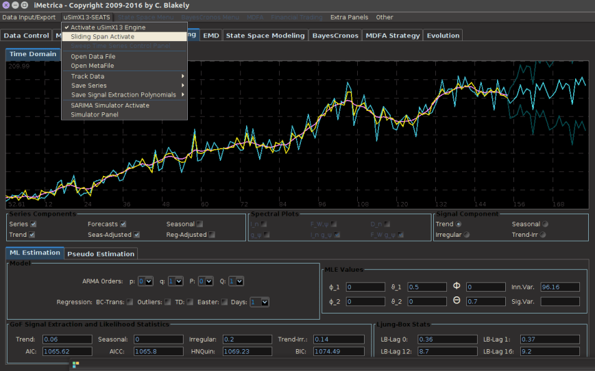
With the uSimX13 engine activated, this essentially turns on all the automatic estimation components of X-13-AS. The original data will be plotted in cyan, while all the extraction signals will be accessible through clicking on the checkbars in the control panel. One can change the modeling SARIMA dimensions, add outlier or other regression detection components, and visualize automatically the changes in the extracted components. All signal extraction and goodness-of-fit diagnoistcs are shown on the bottom of the control panel.
Once the data has been loaded in, one exploratory feature on the module is the ‘Sliding Span Activate’ that offers a unique approach to model selection and goodness-of-fit by addressing multi-step ahead forecasting error on ‘test’ portions of the data. Such analysis can be readily achieved by using the ‘Sliding Span Activate’ component along with the ‘Sweep Time Series Control Panel’. Further details of this interactive model selection feature can be found in one of my previous articles on model selection here.
That will get you started with the basic features in loading data into the model. To learn more, click on the .pdf file here usimx13 for a full guide on how to use all the components in the uSimX13, including a quick guide on the inference of model selection with signal extraction goodness-of-fit diagnostics that was featured in a recent paper by myself and colleague Tucker McElroy here .
Coming next week: Interactive modeling with State Space and RegComponent models using the State Space Modeling module in iMetrica.
