Animation 1: Click to see animation of the Japanese Yen filter in action on 164 hourly out-of-sample observations.
I recently acquired over 300 GBs of financial data that includes tick data for over 7000 financial assets traded on multiple markets for the past 5 years up until February 1st 2013. This USB drive packed with nearly every detail of world financial markets coupled with iMetrica gave me an opportunity to explore at any fashion to my desire the ability of multivariate direct filtering to produce high performance financial trading signals on nearly any high-frequency. Let me begin this article with saying that I am more than ecstatic with the results, as I hope you will too after reading this article. In this first article in a series of high-frequency trading with MDFA and iMetrica that I plan to write, I provide some initial experiments with building and extracting financial trading signals for high-frequency intraday observations on foreign exchange (FOREX) data, and by high-frequency in the context of this article, I mean higher frequencies than the daily log-returns I’ve been working with in my previous articles. In the first part of this high-frequency series, I begin by exploring hourly, 30 minute, and 15 minute log-returns, and test different strategies, mostly using low-pass and the recently introduced multi-bandpass (MBP) filter to deduce the best approach to tackle the problem of building successful trading signals in higher frequency data.
In my previous articles, I was working uniquely with daily log-return data from different time spans from a year to a year and a half. This enabled the in-sample period of computing the filter coefficients for the signal extraction to include all the most recent annual phases and seasons of markets, from holiday effects, to the transitioning period of August to September that is regularly highly influential on stock market prices and commodities as trading volume increases a significant amount. One immediate question that is raised in migrating to higher-frequency intraday data is what kind of in-sample/out-of-sample time spans should be used to compute the filter in-sample and then for how long do we apply the filter out-of-sample to produce the trades? Another question that is raised with intraday data is how do we account for the close-to-open variation in price? Certainly, after close, the after-hour bids and asks will force a jump into the next trading day. How do we deal with this jump in an optimal manner? As the observation frequency gets higher, say from one hour to 30 minutes, this close-to-open jump/fall should most likely be larger. I will start by saying that, as you will see in the results of this article, with a clever choice of the extractor  and explanatory series, MDFA can handle these jumps beautifully (both aesthetically and financially). In fact, I would go so far as to say that the MDFA does a superb job in predicting the overnight variation.
One advantage of building trading signals for higher intraday frequencies is that the signals produce trading strategies that are immediately actionable. Namely one can act upon a signal to enter a long or short position immediately when they happen. In building trading signals for the daily log-return, this is not the case since the observations are not actionable points, namely the log difference of today’s ending price with yesterday’s ending price are produced after hours and thus not actionable during open market hours and only actionable the next trading day. Thus trading on intraday observations can lead to better efficiency in trading.
In this first installment in my series on high-frequency financial trading using multivariate direct filtering in iMetrica, I consider building trading signals on hourly returns of foreign exchange currencies. I’ve received a few requests after my recent articles on the Frequency Effect in seeing iMetrica and MDFA in action on the FOREX sector. So to satisfy those curiosities, I give a series of (financially) satisfying and exciting results in combining MDFA and the FOREX. I won’t give all my secretes away into building these signals (as that would of course wipe out my competitive advantage), but I will give some of the parameters and strategies used so any courageously curious reader may try them at home (or the office). In the conclusion, I give a series of even more tricks and hacks. The results below speak for themselves So without further ado, let the games begin.
Japanese Yen
Frequency: One hour returns
30 day out-of-sample ROI: 12 percent
Trade success ratio: 92 percent
Yen Filter Parameters:  = 9.2
= 9.2  = 13.2,
Regularization: smooth = .918, decay = .139, decay2 = .79, cross = 0
In the first experiment, I consider hourly log-returns of a ETF index that mimics the Japanese Yen called FXY. As for one of the explanatory series, I consider the hourly log-returns of the price of GOLD which is traded on NASDAQ. The out-of-sample results of the trading signal built using a low-pass filter and the parameters above are shown in Figure 1. The in-sample trading signal (left of cyan line) was built using 400 hourly observations of the Yen during US market hours dating back to 1 October 2012. The filter was then applied to the out-of-sample data for 180 hours, roughly 30 trading days up until Friday, 1 February 2013.
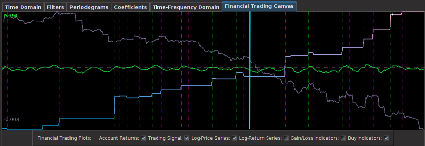
Figure 1: Out-of-sample results for the Japanese Yen. The in-sample trading signal was built using 400 hourly observations of the Yen during US market hours dating back to October 1st, 2012. The out-of-sample portion passed the cyan line is on 180 hourly observations, about 30 trading days.
This beauty of this filter is that it yields a trading signal exhibiting all the characteristics that one should strive for in building a robust and successful trading filter.
- Consistency: The in-sample portion of the filter performs exactly as it does out-of-sample (after cyan line) in both trade success ratio and systematic trading performance.
- Dropdowns: One small dropdown out-of-sample for a loss of only .8 percent (nearly the cost of the transaction).
- Detects the cycles as it should: Although the filter is not able to pinpoint with perfect accuracy every local small upturn during the descent of the Yen against the dollar, it does detect them nonetheless and knows when to sell at their peaks (the magenta lines).
- Self-correction: What I love about a robust filter is that it will tend to self-correct itself very quickly to minimize a loss in an erroneous trade. Notice how it did this in the second series of buy-sell transactions during the only loss out-of-sample. The filter detects momentum but quickly sold right before the ensuing downfall. My intuition is that only frequency-based methods such as the MDFA are able to achieve this consistently. This is the sign of a skillfully smart filter.
The coefficients for this Yen filter are shown below. Notice the smoothness of the coefficients from applying the heavy smooth regularization and the strong decay at the very end. This is exactly the type of smooth/decay combo that one should desire. There is some obvious correlation between the first and second explanatory series in the first 30 lags or so as well. The third explanatory series seems to not provide much support until the middle lags .
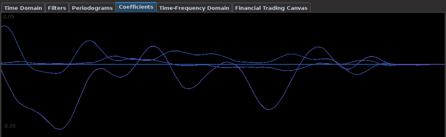
Figure 2: Coefficients of the Yen filter. Here we use three different explanatory series to extract the trading signal.
One of the first things that I always recommend doing when first attempting to build a trading signal is to take a glance at the periodogram. Figure 2 shows the periodogram of the log-return data of the Japanese Yen over 580 hours. Compare this with the periodogram of the same asset using log-returns of daily data over 580 days, shown in Figure 3. Notice the much larger prominent spectral peaks at the lower frequencies in the daily log-return data. These prominent spectral peaks renders multibandpass filters much more advantageous and to use as we can take advantage of them by placing a band-pass filter directly over them to extract that particular frequency (see my article on multibandpass filters). However, in the hourly data, we don’t see any obvious spectral peaks to consider, thus I chose a low-pass filter and set the cutoff frequency at $\pi/5$, a standard choice, and good place to begin.
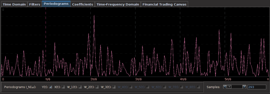
Figure 3: Periodogram of hourly log-returns of the Japanese Yen over 580 hours.
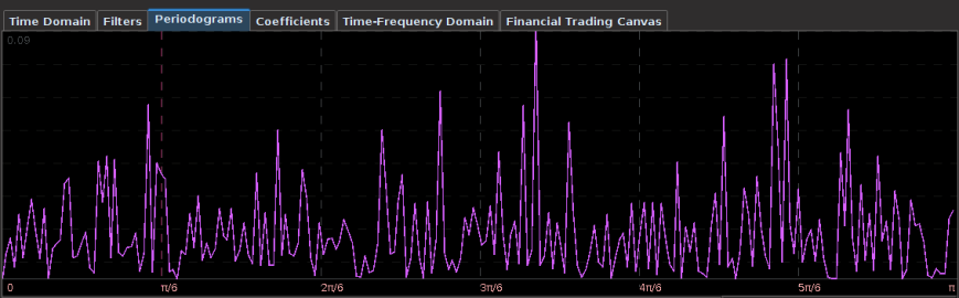
Figure 4: Periodogram of Japanese Yen using 580 daily log-return observations. Many more spectral peaks are present in the lower frequencies.
Japanese Yen
Frequency: 15 minute returns
7 day out-of-sample ROI: 5 percent
Trade success ratio: 82 percent
Yen Filter Parameters: = 3.7 = 13, 
Regularization: smooth = .90, decay = .11, decay2 = .09, cross = 0
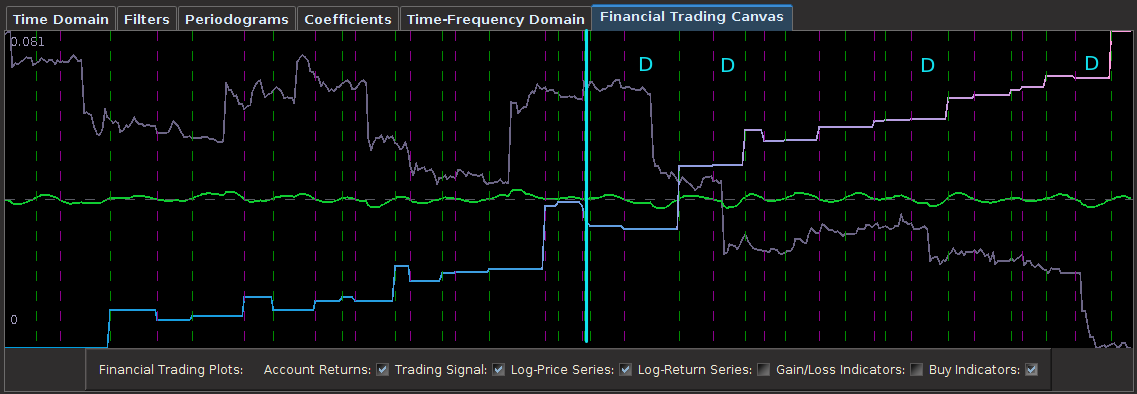
In the next trading experiment, I consider the Japanese Yen again, only this time I look at trading on even high-frequency log-return data than before, namely on 15 minute log-returns of the Yen from the opening bell to market close. This presents slightly new challenges than before as the close-to-open jumps are much larger than before, but these larger jumps do not necessarily pose problems for the MDFA. In fact, I look to exploit these and take advantage to gain profit by predicting the direction of the jump. For this higher frequency experiment, I considered 350 15-minute in-sample observations to build and optimize the trading signal, and then applied it over the span of 200 15-minute out-of-sample observations. This produced the results shown in the Figure 5 below. Out of 17 total trades out-of-sample, there were only 3 small losses each less than .5 percent drops and thus 14 gains during the 200 15-minute out-of-sample time period. The beauty of this filter is its impeccable ability to predict the close-to-open jump in the price of the Yen. Over the nearly 7 day trading span, it was able to correctly deduce whether to buy or short-sell before market close on every single trading day change. In the figure below, the four largest close-to-open variation in Yen price is marked with a “D” and you can clearly see how well the signal was able to correctly deduce a short-sell before market close. This is also consistent with the in-sample performance as well, where you can notice the buys and/or short-sells at the largest close-to-open jumps (notice the large gain in the in-sample period right before the out-of-sample period begins, when the Yen jumped over 1 percent over night. This performance is most likely aided by the explanatory time series I used for helping predict the close-to-open variation in the price of the Yen. In this example, I only used two explanatory series (the price of Yen, and another closely related to the Yen).
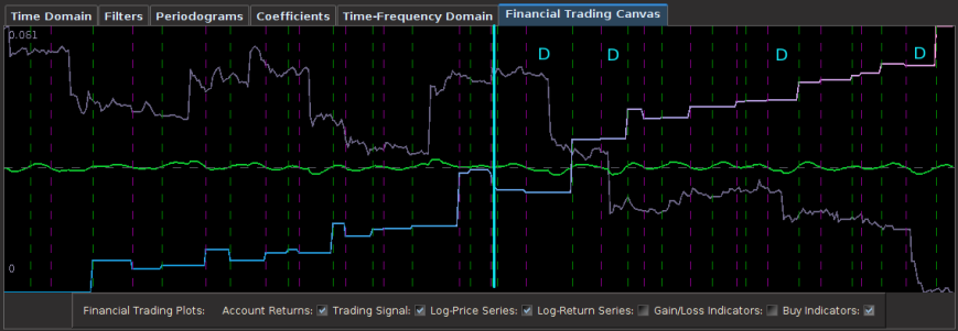
Figure 5: Out-of-sample performance of the Japanese Yen filter on 15 minute log-return data.
We look at the filter transfer functions to see what frequencies they are being privileged in the construction of the filter. Notice that some noise leaks out passed the frequency cutoff at  , but this is typically normal and a non-issue. I had to balance for both timeliness and smoothness in this filter using both the customization parameters and . Not much at frequency 0 is emphasized, with more emphasis stemming from the large spectral peak found right at .
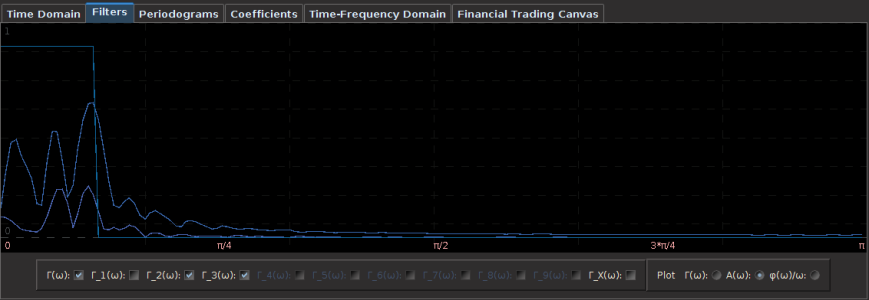
Figure 6: The filter transfer functions.
British Pound
Frequency: 30 minute returns
14 day out-of-sample ROI: 4 percent
Trade success ratio: 76 percent
British Pound Filter Parameters: = 5 = 15,
Regularization: smooth = .109, decay = .165, decay2 = .19, cross = 0
In this example we consider the frequency of the data to 30 minute returns and attempt to build a robust trading signal for a derivative of the British Pound (BP) on this higher frequency. Instead of using the cash value of the BP, I use 30 minute returns of the BP Futures contract expiring in March (BPH3). Although I don’t have access to tick data from the FOREX, I do have tick data from GLOBEX for the past 5 years. Thus the futures series won’t be an exact replication of the cash price series of the BP, but it should be quite close due to very low interest rates.
The results of the out-of-sample performance of the BP futures filter are shown in Figure 7. I constructed the filter using an initial in-sample size of 390 30 minute returns dating back to 1 December 2012. After pinpointing a frequency cutoff in the frequency domain for the that yielded decent trading results in-sample, I then proceeded to optimize the filter in-sample on smoothness and regularization to achieve similar out-of-sample performance. Applying the resulting filter out-of-sample on 168 30-minute log-return observations of the BP futures series along with 3 explanatory series, I get the results shown below. There were 13 trades made and 10 of them were successful. Notice that the filter does an exquisite job at triggering trades near local optimums associated with the frequencies inside the cutoff of the filter.
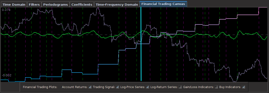
Figure 7: The out-of-sample results of the British Pound using 30-minute return data.
In looking at the coefficients of the filter for each series in the extraction, we can clearly see the effects of the regularization: the smoothness of the coefficients the fast decay at the very end. Notice that I never really apply any cross regularization to stress the latitudinal likeliness between the 3 explanatory series as I feel this would detract from the predicting advantages brought by the explanatory series that I used.
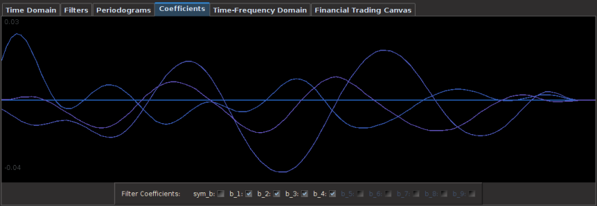
Figure 8: The coefficients for the 3 explanatory series of the BP futures,
Euro
Frequency: 30 min returns
30 day out-of-sample ROI: 4 percent
Trade success ratio: 71 percent
Euro Filter Parameters: = 0, = 6.4,
Regularization: smooth = .85, decay = .27, decay2 = .12, cross = .001
Continuing with the 30 minute frequency of log-returns, in this example I build a trading signal for the Euro futures contract with expiration on 18 March 2013 (UROH3 on the GLOBEX). My in-sample period, being the same as my previous experiment, is from 1 December 2012 to 4 January 2013 on 30 minute returns using three explanatory time series. In this example, after inspecting the periodogram, I decided upon a low-pass filter with a frequency cutoff of . After optimizing the customization and applying the filter to one month of 30 minute frequency return data out-of-sample (month of January 2013, after cyan line) we see the performance is akin to the performance in-sample, exactly what one strives for. This is due primarily to the heavy regularization of the filter coefficients involved. Only four very small losses of less than .02 percent are suffered during the out-of-sample span that includes 10 successful trades, with the losses only due to the transaction costs. Without transaction costs, there is only one loss suffered at the very beginning of the out-of-sample period.
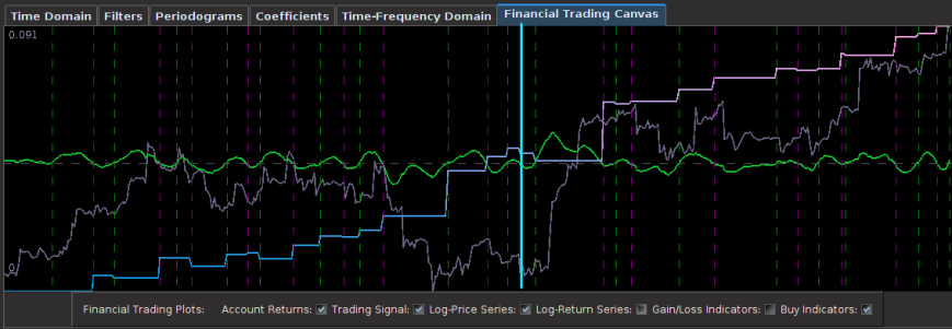
Figure 9 : Out-of-sample performance on the 30-min log-returns of Euro futures contract UROH3.
As in the first example using hourly returns, this filter again exhibits the desired characteristics of a robust and high-performing financial trading filter. Notice the out-of-sample performance behaves akin to the in-sample performance, where large upswings and downswings are pinpointed to high-accuracy. In fact, this is where the filter performs best during these periods. No need for taking advantage of a multibandpass filter here, all the profitable trading frequencies are found at less than . Just as with the previous two experiments with the Yen and the British Pound, notice that the filter cleanly predicts the close-to-open variation (jump or drop) in the futures value and buys or sells as needed. This can be seen from many of the large jumps in the out-of-sample period (after cyan line).
One reason why these trading signals perform so well is due to their approximation power of the symmetric filter. In comparing the trading signal (green) with a high-order approximation of the symmetric filter (gray line) transfer function shown in Figure 10, we see that trading signal does an outstanding job at approximating the symmetric filter uniformly. Even at the latest observation (the right most point), the asymmetric filter hones in on the symmetric signal (gray line) with near perfection. Most importantly, the signal crosses zero almost exactly where required. This is exactly what you want when building a high-performing trading signal.
Figure 10: Plot of approximation of the real-time trading signal for UROH3 with a high order approximation of the symmetric filter transfer function.
In looking at the periodogram of the log-return data and the output trading signal differences (colored in blue), we see that the majority of the frequencies were accounted for as expected in comparing the signal with the symmetric signal. Only an inconsequential amount of noise leakage passed the frequency cutoff of is found. Notice the larger trading frequencies, the more prominent spectral peaks, are located just after  . These could be taken into account with a smart multibandpass filter in order to manifest even more trades, but I wanted to keep things simple for my first trials with high-frequency foreign exchange data. I’m quite content with the results that I’ve achieved so far.
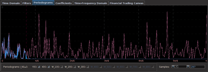
Figure 11: Comparing the periodogram of the signal with the log-return data.
Conclusion
I must admit, at first I was a bit skeptical of the effectiveness that the MDFA would have in building any sort of successful trading signal for FOREX/GLOBEX high frequency data. I always considered the FOREX market rather ‘efficient’ due to the fact that it receives one of the highest trading volumes in the world. Most strategies that supposedly work well on high-frequency FOREX all seem to use some form of technical analysis or charting (techniques I’m particularly not very fond of), most of which are purely time-domain based. The direct filter approach is a completely different beast, utilizing a transformation into the frequency domain and a ‘bending and warping’ of the metric space for the filter coefficients to extract a signal within the noise that is the log-return data of financial assets. For the MDFA to be very effective at building timely trading signals, the log-returns of the asset need to diverge from white noise a bit, giving room for pinpointing intrinsically important cycles in the data. However, after weeks of experimenting, I have discovered that building financial trading signals using MDFA and iMetrica on FOREX data is as rewarding as any other.
As my confidence has now been bolstered and amplified even more after my experience with building financial trading signals with MDFA and iMetrica for high-frequency data on foreign exchange log-returns at nearly any frequency, I’d be willing to engage in a friendly competition with anyone out there who is certain that they can build better trading strategies using time domain based methods such as technical analysis or any other statistical arbitrage technique. I strongly believe these frequency based methods are the way to go, and the new wave in financial trading. But it takes experience and a good eye for the frequency domain and periodograms to get used to. I haven’t seen many trading benchmarks that utilize other types of strategies, but i’m willing to bet that they are not as consistent as these results using this large of an out-of-sample to in-sample ratio (the ratios in these experiments were between .50 and .80). If anyone would like to take me up on my offer for a friendly competition (or know anyone that would), feel free to contact me.
After working with a multitude of different financial time series and building many different types of filters, I have come to the point where I can almost eyeball many of the filter parameter choices including the most important ones being the extractor along with the regularization parameters, without resorting to time consuming, and many times inconsistent, optimization routines. Thanks to iMetrica, transitioning from visualizing the periodogram to the transfer functions and to the filter coefficients and back to the time domain to compare with the approximate symmetric filter in order to gauge parameter choices is an easy task, and an imperative one if one wants to build successful trading signals using MDFA.
Here are some overall tips and tricks to build your own high performance trading signals on high-frequency data at home:
- Pay close attention to the periodogram. This is your best friend in choosing the extractor . The best performing signals are not the ones that trade often, but trade on the most important frequencies found in the data. Not all frequencies are created equal. This is true when building either low-pass or multibandpass frequencies.
- When tweaking customization, always begin with , the parameter for smoothness. for timeliness should be the last resort. In fact, this parameter will most likely be next to useless due to the fact that the log-return of financial data is stationary. You probably won’t ever need it.
- You don’t need many explanatory series. Like most things in life, quality is superior to quantity. Using the log-return data of the asset you’re trading along with one and maybe two explanatory series that somewhat correlate with the financial asset you’re trading on is sufficient. Anymore than that is ridiculous overkill, probably leading to over-fitting (even the power of regularization at your fingertips won’t help you).
In my next article, I will continue with even more high-frequency trading strategies with the MDFA and iMetrica where I will engage in the sector of Funds and ETFs. If any curious reader would like even more advice/hints/comments on how to build these trading signals on high-frequency data for the FOREX (or the coefficients built in these examples), feel free to get in contact with me via email. I’ll be happy to help.
Happy extracting!


 -th observation where n is some number much less than the total number of observations $latex N$ in the data set (say, one third the amount). The data sweep then computes the sliding window from
  , in increments of one (see Figure 3). At each addition to the length of the window, the forecast is computed for up to 24 steps ahead. Of course, since the true time series data is known in the out-of-sample region of computation, we can compute the forecast error for up to
  steps ahead and sum up these errors as
  is the default). Lastly, select how many forecast steps you’d like to use in computing the forecast error (1-24). Once content with the settings, click the “Compute time series sweep” button and watch as the window span increases from
  from a SARIMA model of dimension
  , namely a seasonal auto-regressive integrated moving-average process with two non-seasonal moving-average parameters, and one seasonal moving average parameter. The data sweep is performed on the simulated data with a forecast error horizon of length 23 using three different SARIMA models, (a)
  , (b)
, (b)  , (c)
, (c) 


