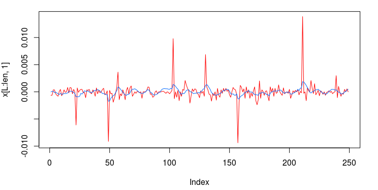
High-Frequency Financial Trading with Multivariate Direct Filtering Part Deux: Index Futures

Posted on February 28, 2013 by Christian Dallas Blakely

Out-of-sample performance (cash, blue-to-pink line) of an MDFA low-pass filter built using the approach discussed in this article on the STOXX Europe 50 index futures with expiration March 18th (STXEH3) for 200 15-minute interval log-return observations. Only one small loss out-of-sample was recorded from the period of Jan 18th through February 1st, 2013.

Continuing along the trend of my previous installment on strategies and performances of high-frequency trading using multivariate direct filtering, I take on building trading signals for high-frequency index futures, where I will focus on the STOXX Europe 50 Index, S&P 500, and the Australian Stock Exchange Index. As you will discover in this article, these filters that I build using MDFA in iMetrica have yielded some of the best performing trading signals that I have seen using any trading methodology. My strategy as I’ve been developing throughout my previous articles on MDFA has not changed much, except for one detail that I will discuss throughout and will be a major theme of this article, and that relates to an interesting structure found in index futures series for intraday returns. The structure is related to the close-to-open variation in the price, namely when the price at close of market hours significantly differs from the price at open. an effect I’ve mentioned in my previous two articles dealing with high(er)-frequency (or intraday) log-return data. I will show how MDFA can take advantage of this variation in price and profit from each one by ‘predicting’ with the extracted signal the jump or drop in the price at the open of the next trading day.

The frequency of observations on the index that are to be considered for building trading filters using MDFA is typically only a question of taste and priorities. The beauty of MDFA lies in not only the versatility and strength in building trading signals for virtually any financial trading priorities, but also in the independence on the underlying observation frequency of the data. In my previous articles, I’ve considered and built high-performing strategies for daily, hourly, and 15 minute log returns, where the focus of the strategy in building the signal began with viewing the periodogram as the main barometer in searching for optimal frequencies on which one should set the low-pass cutoff for the extracting target filter $\Gamma$ function.

Index futures, as in a futures contract on a financial index, as we will see in this article present no new challenges. With the success I had on the 15-minute return observation frequency that I utilized in my previous article in building a signal for the Japanese Yen, I will continue to use the 15 minute intervals for the index futures where I hope to shed some more light on the filter selection process. This includes deducing properties of the intrinsically optimal spectral peaks to trade on. To do this, I present a simple approach I take in these examples by first setting up a bandpass filter over the spectral peak in the periodogram and then study the in-sample and out-of-sample characteristics of this signal, both in performance and consistency. So without further ado, I present my experiments with financial trading on index futures using MDFA, in iMetrica.

STOXX Europe 50 Index (STXE H3, Expiration March 18 2013)

The STOXX Europe 50 Index, Europe’s leading Blue-chip index, provides a representation of sector leaders in Europe. The index covers 50 stocks from 18 European countries and has the highest trading volume of any European index. One of the first things to notice with the 15-minute log-returns of STXE are the frequent large spikes. These spikes will occur every 27 observations at 13:30 (UTC time zone) due to the fact that there are 26 15-minute periods during the trading hours. These spikes represent the close-to-open jumps that the STOXX Europe 50 index has been subjected to and then reflected in the price of the futures contract. With this ‘seasonal’ pattern so obviously present in the log-return data, the frequency effects of this pattern should be clearly visible in the periodogram of the data. The beauty of MDFA (and iMetrica) is that we have the ability to explicitly engineer a trading signal to take advantage of this ‘seasonal’ pattern by building an appropriate extractor $\Gamma$ .

Figure 1: Log-returns of STXE for the 15-min observations from 1-4-2013 to 2-1-2013

Regarding the periodogram of the data, Figure 2 depicts the periodograms for the 15 minute log-returns of STXE (red) and the explanatory series (pink) together on the same discretized frequency domain. Notice that in both log-return series, there is a principal spectral peak found between .23 and .32. The trick is to localize the spectral peak that accounts for the cyclical pattern that is brought about by the close-to-open variation between 20:00 and 13:30 UTC.

Figure 2: The periodograms for the 15 minute log-returns of STXE (red) and the explanatory series (pink).

In order to see the effects of the MDFA filter when localizing this spectral peak, I use my target $\Gamma$ builder interface in iMetrica to set the necessary cutoffs for the bandpass filter directly covering both spectral peaks of the log-returns, which are found between .23 and .32. This is shown in Figure 3, where the two dashed red lines show indicate the cutoffs and spectral peak is clearly inside these two cutoffs, with the spectral peak for both series occurring in the vicinity of $\pi/12$ . Once the bandpass target $\Gamma$ was fixed on this small frequency range, I set the regularization parameters for the filter coefficients to be $\lambda_{smooth} = .86$ , $\lambda_{decay} = .11$ , and $\lambda_{decay2} = .11$ .

Figure 3: Choosing the cutoffs for the band pass filter to localize the spectral peak.

Pinpointing this frequency range that zooms in on the largest spectral peak generates a filter that acts on the intrinsic cycles found in the 15 minute log-returns of the STXE futures index. The resulting trading signal produced by this spectral peak extraction is shown in Figure 4, with the returns (blue to pink line) generated from the trading signal (green) , and the price of the STXE futures index in gray. The cyclical effects in the signal include the close-to-open variations in the data. Notice how the signal predicts the variation of the close-to-open price in the index quite well, seen from the large jumps or falls in price every 27 observations. The performance of this simple design in extracting the spectral peak of STXE yields a 4 percent ROI on 200 observations out-of-sample with only 3 losses out of 20 total trades (85 percent trade success rate), with two of them being accounted for towards the very end of the out-of-sample observations in an uncharacteristic volatile period occurring on January 31st 2013.

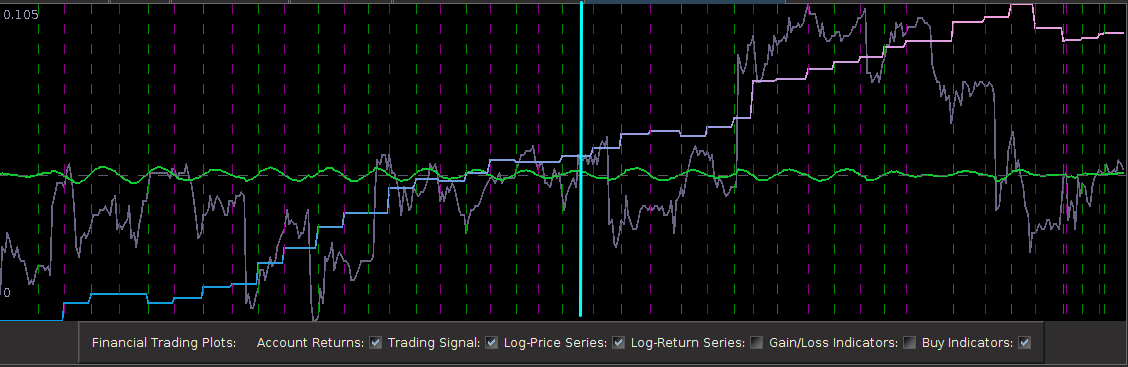
Figure : The performance in-sample and out-of-sample of the spectral peak localizing bandpass filter.

Figure 4: The performance in-sample and out-of-sample of the spectral peak localizing bandpass filter.

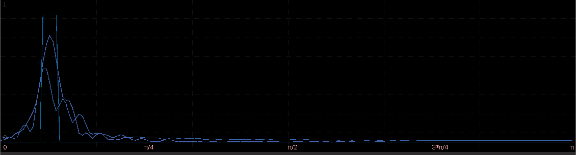
The two concurrent frequency response (transfer) functions for the two filters acting on the STXE log-return data (purple) and the explanatory series (blue), respectively, are plotted below in Figure 5. Notice the presence of the spectral peaks for both series being accounted for in the vicinity of the frequency $\pi/12$ , with mild damping at the peak. Slow damping of the noise in the higher frequencies is aided by the addition of a smoothing expweight parameter that was set at $\alpha = 4$ .

Figure 5: The concurrent frequency response functions of the localizing spectral peak band-pass filter.

With the ideal characteristics of a trading signal quite present in this simple bandpass filter, namely smooth decaying filter coefficients, in-sample and out-of-sample performance properties identical, and accurate, consistent trading patterns, it would be hard to imagine on improving the trading signal for this European futures index even more. But we can. We simply keep the spectral peak frequencies intact, but also account for the local bias in log-return data by extending the lower cutoff to frequency zero. This will provide improved systematic trading characteristics by not only predicting the close-to-open variation and jumps, but also handling upswings and downswings, and highly volatile periods much better.

In this new design, I created a low-pass filter by keeping the upper cutoff $\omega_1$ from the band-pass design and setting the lower cutoff to 0. I also increased the smoothing parameter to $\alpha = 32$. In this newly designed filter, we see a vast improvement in the trading structure. As before, the filter was able to deduce the direction of every single close-to-open jump during the 200 out-of-sample observations, but notice that it was also able to become much more flexible in the trading during any upswing/downswing and volatile period. This is seen in more detail in Figure 7, where I added the letter ‘D’ to each of the 5 major buy/sell signals occurring before close.

Figure : Performance of filter both in-sample (left of cyan line) and on 210 observations out-of-sample (right of cyan line).

Figure 6: Performance of filter both in-sample (left of cyan line) and on 210 observations out-of-sample (right of cyan line).

Notice that the signal predicted the jump correctly for each of these major jumps, resulting in large returns. For example, at the first “D” indicator, the signal indicated sell/short (magenta dashed line) the STXE future index 5 observations before close, namely at 18:45 UTC, before market close at 20:00 UTC. Sure enough, the price of the STXE contract went down during overnight trading hours and opened far below the previous days close, with the filter signaling a buy (green dashed line) 45 minutes into trading. At the mark of the second “D”, we see that on the final observation before market close, the signal produced a buy/long indication, and indeed, the next day the price of the future jumped significantly.

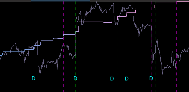
Figure : Zooming in on the out-of-sample performance and showing all the signal responses that predicted the major close-to-open jumps.

Figure 7: Zooming in on the out-of-sample performance and showing all the signal responses that predicted the major close-to-open jumps.

Only two very small losses of less than .08 percent were accounted for. One advantage of including the frequency zero along with the spectral peak frequency of STXE is that the local bias can help push-up or pull-down the signal resulting in a more ‘patient’ or ‘diligent’ filter that can better handle long upswings/downswings or volatile periods. This is seen in the improvement of the performance towards the end of the 200 observations out-of-sample, where the filter is more patient in signaling a sell/short after the previous buy. Compare this with the end of the performance from the band-pass filter, Figure 4. With this trading signal out-of-sample, I computed a 5 percent ROI on the 200 observations out-of-sample with only 2 small losses. The trading statistics for the entire in-sample combined with out-of-sample are shown in Figure 8.

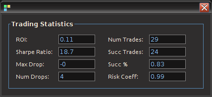
Figure 9: The total performance statistics of the STXEH3 trading signal in-sample plus out-of-sample.

Figure 8: The total performance statistics of the STXEH3 trading signal in-sample plus out-of-sample. The max drop indicates -0 due to the fact that there was a truncation to two decimal places. Thus the losses were less than .01.

S&P 500 Futures Index (ES H3, Expiration March 18 2013)

In this experiment trading S&P 500 future contracts (E-mini) on observations of 15 minute intervals from Jan 4th to Feb 1st 2013, I apply the same regimental approach as before. In looking at the log-returns of ESH3 shown in Figure 10, the effect of close-to-open variation seem to be much less prominent here compared to that on the STXE future index. Because of this, the log-returns seem to be much closer to ‘white noise’ on this index. Let that not perturb our pursuit of a high performing trading signal however. The approach I take for extracting the trading signal, as always, begins with the periodogram.

Figure 10: The log-return data of ES H3 at 15 minute intervals from 1-4-2013 to 2-1-2013.

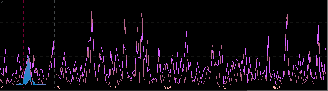
As the large variations in the close-to-open price are not nearly as prominent, it would make sense that the same spectral peak found before at near $\pi/12$ is not nearly as prominent either. We can clearly see this in the periodogram plotted below in Figure 11. In fact, the spectral peak at $\pi/12$ is slightly larger in the explanatory series (pink), thus we should still be able to take advantage of any sort of close-to-open variation that exists in the E-min future index.

Figure 13: Periodograms of ES H3 log-returns (red) and the explanatory series (pink). The red dashed vertical lines are framing the spectral peak between .23 and .32.

Figure 11: Periodograms of ES H3 log-returns (red) and the explanatory series (pink). The red dashed vertical lines are framing the spectral peak between .23 and .32.

With this spectral peak extracted from the series, the resulting trading signal is shown in Figure 12 with the performance of the bandpass signal shown in Figure 13.

Figure 12: The signal built from the extracted spectral peak and the log-return ESH3 data.

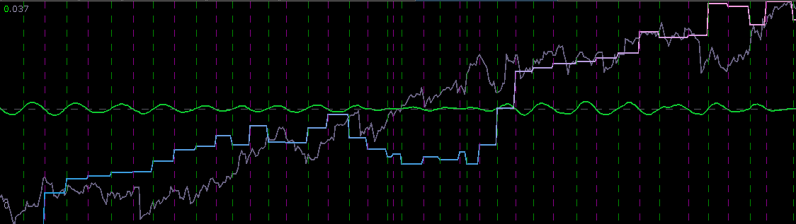
One can clearly see that the trading signal performs very well during the consistent cyclical behavior in the ESH3 price, However, when breakdown occurs in this stochastic structure and follows more prominently another frequency, the trading signal dies and no longer trades systematically taking advantage of the intrinsic cycle found near $\pi/12$ . This can be seen in the middle 90 or so observations. The price can be seen to follow more closely a random walk and the trading becomes inconsistent. After this period of 90 or so observations however, just after the beginning of the out-of-sample period, the trajectory of the ESH3 follows back on its consistent course with a $\pi/12$ cyclical component it had before.

Figure 13: The performance in-sample and out-of-sample of the simple bandpass filter extracting the spectral peak.

Now to improve on these results, we include the frequency zero by moving the lower cutoff of the previous band-pass filter to $\latex \omega_0 = 0$. As I mentioned before, this lifts or pushes down the signal from the local bias and will trade much more systematically. I then lessened the amount of smoothing in the expweight function to $\alpha = 24$ , down from $\alpha = 36$ as I had on the band-pass filter. This allows for slightly higher frequencies than $\pi/12$ to be traded on. I then proceeded to adjust the regularization parameters to obtain a healthy dosage of smoothness and decay in the coefficients. The result of this new low-pass filter design is shown in Figure 14.

Figure 11: Performance out-of-sample (right of cyan line) of the ES H3 filter on 200 15 minute observations.

Figure 14: Performance out-of-sample (right of cyan line) of the ES H3 filter on 200 15 minute observations.

The improvement in the overall systematic trading and performance is clear. Most of the major improvements came from the middle 90 points where the trading became less cyclical. With 6 losses in the band-pass design during this period alone, I was able to turn those losses into two large gains and no losses. Only one major loss was accounted for during the 200 observation out-of-sample testing of filter from January 18th to February 1st, with an ROI of nearly 4 percent during the 9 trading days. As with the STXE filter in the previous example, I was able to successfully build a filter that correctly predicts close-to-open variations, despite the added difficulty that such variations were much smaller. Both in-sample and out-of-sample, the filter performs consistently, which is exactly what one strives for thanks to regularization.

ASX Futures (YAPH3, Expiration March 18, 2013)

In the final experiment, I build a trading signal for the Australian Stock Exchange futures, during the same period of the previous two experiments. The log-returns show moderately large jumps/drops in price during the entire sample from Jan 4th to Feb 1st, but not quite as large as in the STXE index. We still should be able to take advantage of these close-to-open variations.

Figure 15: The log-returns of the YAPH3 in 15-minute interval observations.

In looking at the periodograms for both the YAPH3 15 minute log-returns (red) and the explanatory series (pink), it is clear that the spectral peaks don’t align like they did in the previous two exampls. In fact, there hardly exists a dominant spectral peak in the explanatory series, whereas the $\pi/12$ spectral peak in YAPH3 is very prominent. This ultimately might effect the performance of the filter, and consequently the trades. After building the low-pass filter and setting a high smoothing expweight parameter $\alpha = 26.5$ , I then set the regularization parameters to be $\lambda_{smooth} = .85$ , $\lambda_{decay} = .11$ , and $\lambda_{decay2} = .11$ (same as first example).

Figure : The periodograms for YAPH3 and explanatory series with spectral peak in YAPH3 framed by the red dashed lines.

Figure 16: The periodograms for YAPH3 and explanatory series with spectral peak in YAPH3 framed by the red dashed lines.

The performance of the filter in-sample and out-of-sample is shown in Figure 18. This was one of the more challenging index futures series to work with as I struggled finding an appropriate explanatory series (likely because I was lazy since it was late at night and I was getting tired). Nonetheless, the filter still seems to predict the close-to-open variation on the Australian stock exchange index fairly well. All the major jumps in price are accounted for if you look closely at the trades (green dashed lines are buys/long and magenta lines are sells/shorts) and the corresponding action on the price of the futures contract. Five losses out-of-sample for a trade success ratio of 72 percent and an ROI out-of-sample on 200 observations of 4.2 percent. As with all other experiments in building trading signals with MDFA, we check the consistency of the in-sample and out-of-sample performance, and these seem to match up nicely.

Figure : The out-of-sample performance of the low-pass filter on YAPH3.

Figure 18 : The out-of-sample performance of the low-pass filter on YAPH3.

The filter coefficients for the YAPH3 log-difference series is shown in Figure 19. Notice the perfectly smooth undulating yet decaying structure of the coefficients as the lag increases. What a beauty.

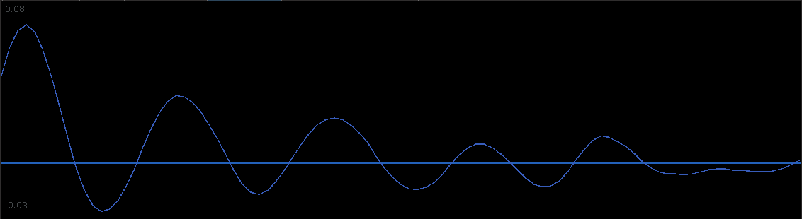
Figure 16: Filter coefficients for the YAPH3 series.

Figure 19: Filter coefficients for the YAPH3 series.

Conclusion

Studying the trading performance of spectral peaks by first constructing band-pass filters to extract the signal corresponding to the peak in these index futures enabled me to understand how I can better construct the lowpass filter to yield even better performance. In these examples, I demonstrated that the close-to-open variation in the index futures price can be seen in the periodogram and thus be controlled for in the MDFA trading signal construction. This trading frequency corresponds to roughly $\pi/12$ in the 15 minute observation data that I had from Jan 4th to Feb 1st. As I witnessed in my empirical studies using iMetrica, this peak is more prominent when the close-to-open variations are larger and more often, promoting a very cyclical structure in the log-return data. As I look deeper and deeper into studying the effects of extracting spectral peaks in the periodogram of financial data log-returns and the trading performance, I seem to improve on results even more and building the trading signals becomes even easier.

Stay tuned very soon for a tutorial using R (and MDFA) for one of these examples on high-frequency trading on index futures. If you have any questions or would like to request a certain index future (out of one of the above examples or another) to be dissected in my second and upcoming R tutorial, feel free to shoot me an email.

Happy extracting!

High-Frequency Financial Trading on FOREX with MDFA and R: An Example with the Japanese Yen

Posted on February 19, 2013 by Christian Dallas Blakely

In-sample (observations 1-235) and out-of-sample (observations 236-455) performance of the trading signal built in this tutorial using MDFA. (Top) The log price of the Yen (FXY) in 15 minute intervals and the trades generated by the trading signal. Here black line is a buy (long), blue is sell (short position). (Bottom) The returns accumulated (cash) generated by the trading, in percentage gained or lossed.

Figure 1: In-sample (observations 1-250) and out-of-sample performance of the trading signal built in this tutorial using MDFA. (Top) The log price of the Yen (FXY) in 15 minute intervals and the trades generated by the trading signal. Here black line is a buy (long), blue is sell (short position). (Bottom) The returns accumulated (cash) generated by the trading, in percentage gained or lost.

In my previous article on high-frequency trading in iMetrica on the FOREX/GLOBEX, I introduced some robust signal extraction strategies in iMetrica using the multidimensional direct filter approach (MDFA) to generate high-performance signals for trading on the foreign exchange and Futures market. In this article I take a brief leave-of-absence from my world of developing financial trading signals in iMetrica and migrate into an uber-popular language used in finance due to its exuberant array of packages, quick data management and graphics handling, and of course the fact that it’s free (as in speech and beer) on nearly any computing platform in the world.

This article gives an intro tutorial on using R for high-frequency trading on the FOREX market using the R package for MDFA (offered by Herr Doktor Marc Wildi von Bern) and some strategies that I’ve developed for generating financially robust trading signals. For this tutorial, I consider the second example given in my previous article where I engineered a trading signal for 15-minute log-returns of the Japanese Yen (from opening bell to market close EST). This presented slightly new challenges than before as the close-to-open jump variations are much larger than those generated by hourly or daily returns. But as I demonstrated, these larger variations on close-to-open price posed no problems for the MDFA. In fact, it exploited these jumps and made large profits by predicting the direction of the jump. Figure 1 at the top of this article shows the in-sample (observations 1-250) and out-of-sample (observations 251 onward) performance of the filter I will be building in the first part of this tutorial.

Throughout this tutorial, I attempt to replicate these results that I built in iMetrica and expand on them a bit using the R language and the implementation of the MDFA available in here. The data that we consider are 15-minute log-returns of the Yen from January 4th to January 17th and I have them saved as an .RData file given by ld_fxy_insamp. I have an additional explanatory series embedded in the .RData file that I’m using to predict the price of the Yen. Additionally, I also will be using price_fxy_insamp which is the log price of Yen, used to compute the performance (buy/sells) of the trading signal. The ld_fxy_insamp will be used as the in-sample data to construct the filter and trading signal for FXY. To obtain this data so you can perform these examples at home, email me and I’ll send you all the necessary .RData files (the in-sample and out-of-sample data) in a .zip file. Taking a quick glance at the ld_fxy_insamp data, we see log-returns of the Yen at every 15 minutes starting at market open (time zone UTC). The target data (Yen) is in the first column along with the two explanatory series (Yen and another asset co-integrated with movement of Yen).
> head(ld_fxy_insamp) [,1] [,2] [,3] 2013-01-04 13:30:00 0.000000e+00 0.000000e+00 0.0000000000 2013-01-04 13:45:00 4.763412e-03 4.763412e-03 0.0033465833 2013-01-04 14:00:00 -8.966599e-05 -8.966599e-05 0.0040635638 2013-01-04 14:15:00 2.597055e-03 2.597055e-03 -0.0008322064 2013-01-04 14:30:00 -7.157556e-04 -7.157556e-04 0.0020792190 2013-01-04 14:45:00 -4.476075e-04 -4.476075e-04 -0.0014685198

Moving on, to begin constructing the first trading signal for the Yen, we begin by uploading the data into our R environment, define some initial parameters for the MDFA function call, and then compute the DFTs and periodogram for the Yen.

load(paste(path.pgm,&quot;ld_fxy_in15min.RData&quot;,sep=&quot;&quot;))    #load in-sample log-returns of Yen
load(paste(path.pgm,&quot;price_fxy_in15min.RData&quot;,sep=&quot;&quot;)) #load in-sample log-price of Yen

in_samp_lenprice_insample&lt;-price_fxy_insamp

#setup some MDFA variables
x&lt;-ld_fxy_insamp
len&lt;-length(x[,1])
shift_constraint&lt;-rep(0,length(x[1,])-1)
weight_constraint&lt;-rep(0,length(x[1,])-1)
d&lt;-0
plots&lt;-T
lin_expweight&lt;-F

# Compute DFTs and periodogram for initial analysis
spec_obj&lt;-spec_comp(len,x,d)
weight_func&lt;-spec_obj$weight_func
K&lt;-length(weight_func[,1])-1
fxy_periodogram&lt;-abs(spec_obj$weight_func[,1])^2

As I’ve mentioned in my previous articles, my step-by-step strategy for building trading signals always begin by a quick analysis of the periodogram of the asset being traded on. Holding the key to providing insight into the characteristics of how the asset trades, the periodogram is an essential tool for navigating how the extractor $\Gamma$ is chosen. Here, I look for principal spectral peaks that correspond in the time domain to how and where my signal will trigger buy/sell trades. Figure 2 shows the periodogram of the 15-minute log-returns of the Japanese Yen during the in-sample period from January 4 to January 17 2013. The arrows point to the main spectral peaks that I look for and provides a guide to how I will define my $\Gamma$ function. The black dotted lines indicate the two frequency cutoffs that I will consider in this example, the first being $\pi/12$ and the second at $\pi/6$ . Notice that both cutoffs are set directly after a spectral peak, something that I highly recommend. In high-frequency trading on the FOREX using MDFA, as we’ll see, the trick is to seek out the spectral peak which accounts for the close-to-open variation in the price of the foreign currency. We want to take advantage of this spectral peak as this is where the big gains in foreign currency trading using MDFA will occur.

Figure 2: Periodogram of FXY (Japanese Yen) along with spectral peaks and two different frequency cutoffs.

In our first example we consider the larger frequency as the cutoff for $\Gamma$ by setting it to $\pi/6$ (the right most line in the figure of the periodogram). I then initially set the timeliness and smoothness parameters, $lambda$ and expweight to 0 along with setting all the regularization parameters to 0 as well. This will give me a barometer for where and how much to adjust the filter parameters. In selecting the filter length $L$ , my empirical studies over numerous experiments in building trading signals using iMetrica have demonstrated that a ‘good’ choice is anywhere between 1/4 and 1/5 of the total in-sample length of the time series data. Of course, the length depends on the frequency of the data observations (i.e. 15 minute, hourly, daily, etc.), but in general you will most likely never need more than $L$ being greater than 1/4 the in-sample size. Otherwise, regularization can become too cumbersome to handle effectively. In this example, the total in-sample length is 335 and thus I set $L= 82$ which I’ll stick to for the remainder of this tutorial. In any case, the length of the filter is not the most crucial parameter to consider in building good trading signals. For a good robust selection of the filter parameters couple with appropriate explanatory series, the results of the trading signal with $L= 80$ compared with, say, $L= 85$ should hardly differ. If they do, then the parameterization is not robust enough.

After uploading both the in-sample log-return data along with the corresponding log price of the Yen for computing the trading performance, we the proceed in R to setting initial filter settings for the MDFA routine and then compute the filter using the IMDFA_comp function. This returns both the i_mdfa& object holding coefficients, frequency response functions, and statistics of filter, along with the signal produced for each explanatory series. We combine these signals to get the final trading signal in-sample. All this is all done in R as follows:


cutoff&lt;-pi/6 #set frequency cutoff
Gamma&lt;-((0:K)&lt;(cutoff*K/pi)) #define Gamma

grand_mean&lt;-F
Lag&lt;-0
L&lt;-82
lambda_smooth&lt;-0
lambda_cross&lt;-0
lambda_decay&lt;-c(0.,0.) #regularization - decay

lambda&lt;-0
expweight&lt;-0
i1&lt;-F
i2&lt;-F
# compute the filter for the given parameter definitions
i_mdfa_obj&lt;-IMDFA_comp(Lag,K,L,lambda,weight_func,Gamma,expweight,cutoff,i1,i2,weight_constraint,
lambda_cross,lambda_decay,lambda_smooth,x,plots,lin_expweight,shift_constraint,grand_mean)

# after computing filter, we save coefficients
bn&lt;-i_mdfa_obj$i_mdfa$b

# now we build trading signal
trading_signal&lt;-i_mdfa_obj$xff[,1] + i_mdfa_obj$xff[,2]

The resulting frequency response functions of the filter and the coefficients are plotted in the figure below.

Figure 3: The Frequency response functions of the filter and the filter coefficients

Figure 3: The Frequency response functions of the filter (top) and the filter coefficients (below)

Notice the abundance of noise still present passed the cutoff frequency. This is mollified by increasing the expweight smoothness parameter. The coefficients for each explanatory series show some correlation in their movement as the lags increase. However, the smoothness and decay of the coefficients leaves much to be desired. We will remedy this by introducing regularization parameters. Plots of the in-sample trading signal and the performance in-sample of the signal are shown in the two figures below. Notice that the trading signal behaves quite nicely in-sample. However, looks can be deceiving. This stellar performance is due in large part to a filtering phenomenon called overfitting. One can deduce that overfitting is the culprit here by simply looking at the nonsmoothness of the coefficients along with the number of freezed degrees of freedom, which in this example is roughly 174 (out of 174), way too high. We would like to get this number at around half the total amount of degrees of freedom (number of explanatory series x L).

Figure 4: The trading signal and the log-return data of the Yen.

The in-sample performance of this filter demonstrates the type of results we would like to see after regularization is applied. But now comes for the sobering effects of overfitting. We apply these filter coeffcients to 200 15-minute observations of the Yen and the explanatory series from January 18 to February 1 2013 and compare with the characteristics in-sample. To do this in R, we first load the out-of-sample data into the R environment, and then apply the filter to the out-of-sample data that I defined as x_out.

load(paste(path.pgm,&quot;ld_fxy_out15min.RData&quot;,sep=&quot;&quot;))
load(paste(path.pgm,&quot;price_fxy_out15min.RData&quot;,sep=&quot;&quot;))
x_out&lt;-rbind(ld_fxy_insamp,ld_fxy_outsamp) #bind the in-sample with out-of-sample data
xff&lt;-matrix(nrow=out_samp_len,ncol=2)

#apply filter built in-sample
for(i in 1:out_samp_len)
{
  xff[i,]&lt;-0
  for(j in 2:3)
  {
      xff[i,j-1]&lt;-xff[i,j-1]+bn[,j-1]%*%x_out[335+i:(i-L+1),j]
  }
}
trading_signal_outsamp&lt;-xff[,1] + xff[,2]     #assemble the trading signal out-of-sample
trade_outsamp&lt;-trading_logdiff(trading_signal_outsamp,price_outsample,.0005)  #compute the performance

The plot in Figure 5 shows the out-of-sample trading signal. Notice that the signal is not nearly as smooth as it was in-sample. Overshooting of the data in some areas is also obviously present. Although the out-of-sample overfitting characteristics of the signal are not horribly suspicious, I would not trust this filter to produce stellar returns in the long run.

Figure : Filter applied to 200 15 minute observations of Yen out-of-sample to produce trading signal (shown in blue)

Figure 5 : Filter applied to 200 15 minute observations of Yen out-of-sample to produce trading signal (shown in blue)

Following the previous analysis of the mean-squared solution (no customization or regularization), we now proceed to clean up the problem of overfitting that was apparent in the coefficients along with mollifying the noise in the stopband (frequencies after $\pi/6$ ). In order to choose the parameters for smoothing and regularization, one approach is to first apply the smoothness parameter first, as this will generally smooth the coefficients while acting as a ‘pre’-regularizer, and then advance to selecting appropriate regularization controls. In looking at the coefficients (Figure 3), we can see that a fair amount of smoothing is necessary, with only a slight touch of decay. To select these two parameters in R, one option is to use the Troikaner optimizer (found here) to find a suitable combination (I have a secret sauce algorithmic approach I developed for iMetrica for choosing optimal combinations of parameters given an extractor $\Gamma$ and a performance indicator, although it’s lengthy (even in GNU C) and cumbersome to use, so I typically prefer the strategy discussed in this tutorial). In this example, I began by setting the lambda_smooth to .5 and the decay to (.1,.1) along with an expweight smoothness parameter set to 8.5. After viewing the coefficients, it still wasn’t enough smoothness, so I proceeded to add more finally reaching .63, which did the trick. I then chose lambda to balance the effects of the smoothing expweight (lambda is always the last resort tweaking parameter).

lambda_smooth&lt;-0.63
lambda_cross&lt;-0.
lambda_decay&lt;-c(0.119,0.099)
lambda&lt;-9
expweight&lt;-8.5

i_mdfa_obj&lt;-IMDFA_comp(Lag,K,L,lambda,weight_func,Gamma,expweight,cutoff,i1,i2,weight_constraint,
lambda_cross,lambda_decay,lambda_smooth,x,plots,lin_expweight,shift_constraint,grand_mean)

bn&lt;-i_mdfa_obj$i_mdfa$b    #save the filter coefficients

trading_signal&lt;-i_mdfa_obj$xff[,1] + i_mdfa_obj$xff[,2]  #compute the trading signal
trade&lt;-trading_logdiff(trading_signal[L:len],price_insample[L:len],0) #compute the in-sample performance

Figure 6 shows the resulting frequency response function for both explanatory series (Yen in red). Notice that the largest spectral peak found directly before the frequency cutoff at $\pi/6$ is being emphasized and slightly mollified (value near .8 instead of 1.0). The other spectral peaks below $\pi/6$ are also present. For the coefficients, just enough smoothing and decay was applied to keep the lag, cyclical, and correlated structure of the coefficients intact, but now they look much nicer in their smoothed form. The number of freezed degrees of freedom has been reduced to approximately 102.

Figure : The frequency response functions and the coefficients after regularization and smoothing have been applied.

Figure 6: The frequency response functions and the coefficients after regularization and smoothing have been applied (top). The smoothed coefficients with slight decay at the end (bottom). Number of freezed degrees of freedom is approximately 102 (out of 172).

Along with an improved freezed degrees of freedom and no apparent havoc of overfitting, we apply this filter out-of-sample to the 200 out-of-sample observations in order to verify the improvement in the structure of the filter coefficients (shown below in Figure 7). Notice the tremendous improvement in the properties of the trading signal (compared with Figure 5). The overshooting of the data has be eliminated and the overall smoothness of the signal has significantly improved. This is due to the fact that we’ve eradicated the presence of overfitting.

Figure : Out-of-sample trading signal with regularization.

Figure 7: Out-of-sample trading signal with regularization.

With all indications of a filter endowed with exactly the characteristics we need for robustness, we now apply the trading signal both in-sample and out of sample to activate the buy/sell trades and see the performance of the trading account in cash value. When the signal crosses below zero, we sell (enter short position) and when the signal rises above zero, we buy (enter long position).

The top plot of Figure 8 is the log price of the Yen for the 15 minute intervals and the dotted lines represent exactly where the trading signal generated trades (crossing zero). The black dotted lines represent a buy (long position) and the blue lines indicate a sell (and short position). Notice that the signal predicted all the close-to-open jumps for the Yen (in part thanks to the explanatory series). This is exactly what we will be striving for when we add regularization and customization to the filter. The cash account of the trades over the in-sample period is shown below, where transaction costs were set at .05 percent. In-sample, the signal earned roughly 6 percent in 9 trading days and a 76 percent trading success ratio.

Figure : In-sample performance of the new filter and the trades that are generated.

Figure 8: In-sample performance of the new filter and the trades that are generated.

Now for the ultimate test to see how well the filter performs in producing a winning trading signal, we applied the filter to the 200 15-minute out-of-sample observation of the Yen and the explanatory series from Jan 18th to February 1st and make trades based on the zero crossing. The results are shown below in Figure 9. The black lines represent the buys and blue lines the sells (shorts). Notice the filter is still able to predict the close-to-open jumps even out-of-sample thanks to the regularization. The filter succumbs to only three tiny losses at less than .08 percent each between observations 160 and 180 and one small loss at the beginning, with an out-of-sample trade success ratio hitting 82 percent and an ROI of just over 4 percent over the 9 day interval.

Figure : Out-of-sample performance of the regularized filter on 200 out-of-sample 15 minute returns of the Yen.

Figure 9: Out-of-sample performance of the regularized filter on 200 out-of-sample 15 minute returns of the Yen. The filter achieved 4 percent ROI over the 200 observations and an 82 percent trade success ratio.

Compare this with the results achieved in iMetrica using the same MDFA parameter settings. In Figure 10, both the in-sample and out-of-sample performance are shown. The performance is nearly identical.

Figure : In-sample and out-of-sample performance of the Yen filter in iMetrica. Nearly identical with performance obtained in R.

Figure 10: In-sample and out-of-sample performance of the Yen filter in iMetrica. Nearly identical with performance obtained in R.

Example 2

Now we take a stab at producing another trading filter for the Yen, only this time we wish to identify only the lowest frequencies to generate a trading signal that trades less often, only seeking the largest cycles. As with the performance of the previous filter, we still wish to target the frequencies that might be responsible to the large close-to-open variations in the price of Yen. To do this, we select our cutoff to be $\pi/12$ which will effectively keep the largest three spectral peaks intact in the low-pass band of $\Gamma$ .

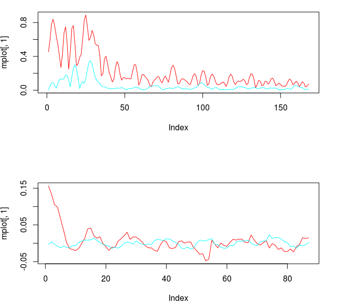
For this new filter, we keep things simple by continuing to use the same regularization parameters chosen in the previous filter as they seemed to produce good results out-of-sample. The $\lambda$ and expweight customization parameters however need to be adjusted to account for the new noise suppression requirements in the stopband and the phase properties in the smaller passband. Thus I increase the smoothing parameter and decreased the timeliness parameter (which only affects the passband) to account for this change. The new frequency response functions and filter coefficients for this smaller lowpass design are shown below in Figure 11. Notice that the second spectral peak is accounted for and only slightly mollified under the new changes. The coefficients still have the noticeable smoothness and decay at the largest lags.

Figure : Frequency response functions of the two filters and their corresponding coefficients.

Figure 11: Frequency response functions of the two filters and their corresponding coefficients.

To test the effectiveness of this new lower trading frequency design, we apply the filter coefficients to the 200 out-of-sample observations of the 15-minute Yen log-returns. The performance is shown below in Figure 12. In this filter, we clearly see that the filter still succeeds in predicting correctly the large close-to-open jumps in the price of the Yen. Only three total losses are observed during the 9 day period. The overall performance is not as appealing as the previous filter design as less amount of trades are made, with a near 2 percent ROI and 76 percent trade success ratio. However, this design could fit the priorities for a trader much more sensitive to transaction costs.

Figure : Out-of-sample performance of filter with lower cutoff.

Figure 12: Out-of-sample performance of filter with lower cutoff.

Conclusion

Verification and cross-validation is important, just as the most interesting man in the world knows.

Verification and cross-validation is important, just as the most interesting man in the world will tell you.

The point of this tutorial was to show some of the main concepts and strategies that I undergo when approaching the problem of building a robust and highly efficient trading signal for any given asset at any frequency. I also wanted to see if I could achieve similar results with the R MDFA package as my iMetrica software package. The results ended up being nearly parallel except for some minor differences. The main points I was attempting to highlight were in first analyzing the periodogram to seek out the important spectral peaks (such as ones associate with close-to-open variations) and to demonstrate how the choice of the cutoff affects the systematic trading. Here’s a quick recap on good strategies and hacks to keep in mind.

Summary of strategies for building trading signal using MDFA in R:

As I mentioned before, the periodogram is your best friend. Apply the cutoff directly after any range of spectral peaks that you want to consider. These peaks are what generate the trades.
Utilize a choice of filter length $L$ no greater than 1/4. Anything larger is unnecessary.
Begin by computing the filter in the mean-square sense, namely without using any customization or regularization and see exactly what needs to be approved upon by viewing the frequency response functions and coefficients for each explanatory series. Good performance of the trading signal in-sample (and even out-of-sample in most cases) is meaningless unless the coefficients have solid robust characteristics in both the frequency domain and the lag domain.
I recommend beginning with tweaking the smoothness customization parameter expweight and the lambda_smooth regularization parameters first. Then proceed with only slight adjustments to the lambda_decay parameters. Finally, as a last resort, the lambda customization. I really never bother to look at lambda_cross. It has seldom helped in any significant manner. Since the data we are using to target and build trading signals are log-returns, no need to ever bother with i1 and i2. Those are for the truly advanced and patient signal extractors, and should only be left for those endowed with iMetrica 😉

If you have any questions, or would like the high-frequency Yen data I used in these examples, feel free to contact me and I’ll send them to you. Until next time, happy extracting!

The Frequency Effect: How to Infer Optimal Frequencies in Financial Trading

Posted on December 31, 2012 by Christian Dallas Blakely

Animation 1: Click to view animation. Periodogram and Various Frequency Intervals.

Animation 2: The in-sample performance of the trading signal for each frequency sweep shown in the animation above.

Animation 2: Click to view the animation. The in-sample performance of the trading signal for each frequency sweep shown in the animation above.

When constructing signals for buy/sell trades in financial data, one of the primary parameters that should be resolved before any other parameters are regarded is the trading frequency structure that regulates all the trades. The structure should be robust and consistent during all regimes of behavior for the given traded asset, namely during times of high volatility, sideways, or bull/bear markets. In the MDFA approach to building trading signals, the trading structure is mostly determined by the characteristics of the target transfer function, the $\Gamma(\omega)$ function that designates the areas of pass and stop-band frequencies in the data. As I argue in this article, I demonstrate that there exists an optimal frequency band in which the trades should be made, and the frequency band is intrinsic to the financial data being analyzed. Two assets do not necessarily share the same optimal frequency band. Needless to say, this frequency band is highly dependent on the frequency of the observations in the data (i.e. minute, hourly, daily) and the type of financial asset. Unfortunately, blindly seeking such an optimal trading frequency structure is a daunting and challenging task in general. Fortunately, I’ve built a few useful tools in the iMetrica financial trading platform to seamlessly navigate towards carving out the best (optimal or at least near optimal) trading frequency structure for any financial trading scenario. I show how it’s done in this article.

We first briefly summarize the procedure for building signals with a targeted range of frequencies in the (multivariate) direct filter approach, and then proceed to demonstrate how it is easily achieved in iMetrica. In order to construct signals of interest in any data set, a target transfer function must first be defined. This target filter transfer function $\Gamma(\omega)$ defined on $\omega \in [0,\pi]$ controls the frequency content of the output signal through the computation of the optimal filter coefficients. 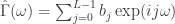Defining $\hat{\Gamma}(\omega) = \sum_{j=0}^{L-1} b_j \exp(i j \omega)$ for some collection of filter coefficients $b_j, \, j=0,\ldots,L-1$ , recall that in the plain-vanilla (univariate) direct filter approach (for ‘quasi’ stationary data), we seek to find the $L$ coefficients such that $\int_{-\pi}^{\pi} |\Gamma(\omega) - \hat{\Gamma}(\omega)|^2 H(\omega) d\omega$ is minimized, where $H(\omega)$ is a ‘smart’ weighting function that approximates the ‘true’ spectral density of the data (in general the periodogram of the data, or a function using the periodogram of the data). By defining $\Gamma(\omega)$ as a function that takes on the value of one or less for a certain range of values in $[0,\pi]$ and zero elsewhere, we pinpoint exotic frequencies where we wish our filter to extract the features of the data. The characteristics of the generated output signal (after the resulting filter has been applied to the data) are those intrinsic to the selected frequencies in the data. The characteristics found at other frequencies are (in a perfect world) disregarded from the output signal. As we show in this article, the selection of the frequencies when defining $\Gamma(\omega)$ provides the utmost in importance when building financial trading signals, as the optimal frequencies in regards to trading performance vary with every data set.

As mentioned, much emphasis should be applied to the construction of this target $\Gamma(\omega)$ and finding the optimal one is not necessarily an easy task in general. With a plethora of other parameters that are involved in building a trading signal, such as customization and regularization (see my article on financial trading parameters), one could just simply select any arbitrary frequency range for $\Gamma(\omega)$ and then proceed to optimize the other parameters until a winning trading signal is found. That is, of course, an option. But I’d like to be an advocate for carving out the proper frequency range that’s intrinsically optimal for the data set given, namely because I believe one exists, and secondly because once in the proper frequency range for the data, other parameters are much easier to optimize. So what kind of properties should this ‘optimal’ frequency range possess in regards to the trading signal?

Consistency. Provides out-of-sample performance akin to in-sample performance.
Optimality. Generates in-sample trade performance with rank coefficient above .90.
Robustness. Insensitive to small changes in parameterization.

Most of these properties are obvious when first glancing at them, but are completely nontrivial to obtain. The third property tends to be overlooked when building efficient trading signals as one typically chooses a parameterization for a specific frequency band in the target $\Gamma(\omega)$ , and then becomes over-confident and optimistic that the filter will provide consistent results out-of-sample. With a non-robust signal, small change in one of the customization parameters completely eradicates the effectiveness and optimality of the filter. An optimal frequency range should be much less sensitive to changes in the customization and regularization of the filter parameters. Namely, changing the smoothing parameter, say 50 percent in either direction, will have little effect on the in-sample performance of the filter, which in turn will produce a more robust signal.

To build a target transfer function $\Gamma(\omega)$ , one has many options in the MDFA module of iMetrica. The approach that we will consider in this article is to define $\Gamma(\omega)$ directly by indicating the frequency pass-band and stop-band structure directly. The simplest transfer functions are defined by two cutoff frequencies: a low cutoff frequency $\omega_0$ and a high-cutoff frequency $\omega_1$ . In the Target Filter Design control panel (see Figure 1), one can control every aspect of the target transfer function $\Gamma(\omega)$ function, from different types of step functions, to more exotic options using modeling. For building financial trading signals, the Band-Pass option will be sufficient. The cutoff frequencies $\omega_0$ and $\omega_1$ are adjusted by simply modifying their values using the slider bars designated for each value, where three different ways of modifying the cutoff frequency values are available. The first is the direct designation of the value using the slider bar which goes between values of $(0,\pi)$ by changes of .01. The second method uses two different slider bars to change the values of the numerator $n$ and denominator $d$ where $\omega_0$ and/or $\omega_1$ is written in fractional form $2\pi n/d$ , a form commonly used for defining different cycles in the data. The third method is to simply type in the value of the cutoff in the designated text area and then press Enter on the keyboard, where the number must be a real number in the interval $(0,\pi)$ and entered in decimal form (i.e. 0.569, 1.349, etc). When the Auto checkbox is selected, the new direct filter and signal will be computed automatically when any changes to the target transfer function are made. This can be a quite useful tool for robustness verification, to see how small changes in the frequency content affect the output signal, and consequently the trading performance of the signal.

Figure 1: Target filter design panel.

Although cycling through multiple frequency ranges to find the optimal frequency bands for in-sample trading performance can be seamlessly accomplished by just sliding the scrollbars around (as shown in Animations 1 and 2 at the top of the page), there is a much easier way to achieve optimality (or near optimality) automatically thanks to a Financial Trading Optimization control panel featured in the Financial Trading menu at the top of the iMetrica interface. Once in the Financial Trading interface, optimization of both the customization parameters for timeliness and smoothness, along with optimization of the $\Gamma(\omega)$ frequency bands can be accomplished by first launching the Trading Optimization panel (see Figure 2), and then selecting the optimization criteria desired (maximum return, minimum loss, maximum trade success ratio, maximum rank coefficient,… etc). 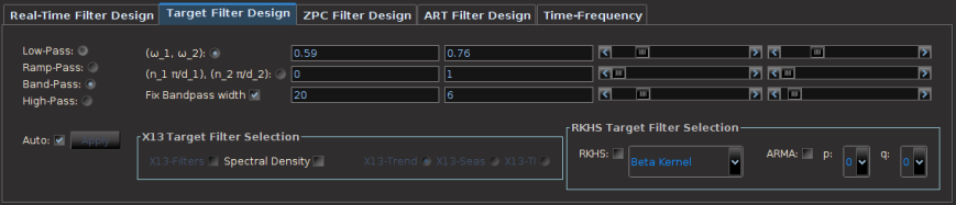To find the optimal customization parameters, simply select the optimization criteria from the drop-down menu, and then click either the Simulated Annealing button, or Grid Search button (as the name implies, ‘grid search’ simply creates a fine grid of customization values $\lambda$ and smoothing expweight $\alpha$ and then chooses the maximal value after sweeping the entire grid – it takes a few seconds depending on the length of the filter. The method that I prefer for now). After the optimal parameters are found, the plotting canvas in the optimization panel paints a contour plot of the values found in order to give you an idea of the customization geometry, with all other parameterization values fixed. The frequency bandwidth of the target transfer function can then be optimized by a quick few millisecond grid search by selecting the checkbox Optimize bandwidth only. In this case the customization parameters are held fixed to their set values, and the optimization proceeds to only vary the frequency parameters. The values of the optimization function produced during the grid-search are then plotted on the optimization canvas to yield the structure from the frequency domain point-of-view. This can be helpful when comparing different frequency bands in building trading signals. It can also help in determining the robustness of the signal, by looking at the near neighboring values found at the optimal value.

Figure 2: The financial trading optimization panel. Here the values of the optimization criteria are plotted for all the different frequency intervals. The interval with the maximum value is automatically chosen and then computed.

We give a full example of an actual trading scenario to show how this process works in selecting an optimal frequency range for a given set of market traded assets. The outline of my general step-by-step approach for seeking good trading filters goes as follows.

Select the initial frequency band-pass by first initializing the $(\omega_1, \omega_2)$ interval to $(0, \omega_2)$ . Setting $\omega_2$ to .10-.15 is usually sufficient. Set the checkbox Fix-Bandpass width in order to secure the bandwidth of the filter.
In the optimization panel (Figure 2), click the checkbox Optimize Bandwidth only and then select the optimization criteria. In these examples, we choose to maximize the rank coefficient, as it tends to produce the best out-of-sample trading performance. Then tap the Grid Search button to find the frequency range with the maximum rank coefficient. This search takes a few milliseconds.
With the initialization of the optimal bandwidth, the customization parameters can now be optimized by deselecting the Optimize Bandwidth only and then tapping the Grid Search button once more. Depending on the length of the filter $L$ and the number of addition explaining series, this search can take several seconds.
Repeat steps 2 and 3 until a combination is found of customization and filter bandwidth that produces a rank coefficient above .90. Also, test the robustness of the trading signal by slightly adjusting the frequency range and the customization parameters by small changes. A robust signal shouldn’t change the trading statistics too much under slight parameter movement.

Once content with the in-sample trading statistics (the Trading Statistics panel is available from the Financial Trading Menu), the final step is to apply the filter to out-of-sample data and trade away. Provided that sufficient regularization parameters have been selected prior to the optimization (regularization selection is out of the scope of this article however) and the optimized trading frequency bandwidth was robust enough, the out-of-sample performance of the signal should perform akin to in-sample. If not, start over with different regularization parameters and filter length, or seek options using adaptive filtering (see my previous article on adaptive filtering).

In our example, we trade on the daily price of GOOG by using GOOG log-return data as the target data and first explanatory series, along with AAPL daily log-returns as the second explanatory series. After the four steps taken above, an optimal frequency range was found to be $(.63,.80)$ , where the in-sample period was from 6-3-2011 to 9-21-2012. The post-optimization of the filter, showing the MDFA trading interface, the in-sample trading statistics, and the trading optimization is shown in Figure 3. Here, the in-sample maximum rank coefficient was found to be at .96 (1.0 is the best, -1.0 is pitiful), where the trade success ratio is around 67 percent, a return-on-investment at 51 percent, and a maximum loss during the in-sample period at around 5 percent. Applying this filter out-of-sample on incoming data for 30 trading days, without any adjustments to the filter, we see that the performance of the signal was very much akin to the performance in-sample (see Figure 5). At the end of the 30 out-of-sample trading days after the in-sample period, the trading signal gives a 65 percent return for a total of a 14 percent return-on-investment in 30 trading days. During this period, there were 6 trades made (3 buys and 3 sell shorts), and 5 of them were successful (with a .1 percent transaction cost for any trade), which amounts to, on average, one trade per week.

Figure 3. After in-sample optimization on both the customization and filter frequency band.

Figure 4: After applying the constructed filter on the next 30 days out-of-sample.

The other filter parameters (customization, regularization, and filter length $L$ ) have been blurred-out on purpose for obvious reasons. However, interested readers can e-mail me and I’ll send the optimal customization and regularization parameters, or maybe even just the filter coefficients themselves so you can apply them to data future GOOG and AAPL data and experiment.) We then apply the filter out-of-sample for 30 days and make trades based on the output of the trading signal. In Figure 4, the blue-to-pink line represents the performance of the trading account given by the percentage returns from each trade made over time. The grey line is the log-price of GOOG, and the green line is the trading signal constructed from the filter just built applied to the data. It signals a ‘buy’ when the signal moves above the zero line (the dotted line) and a sell (and short-sell) when below the line. Since the data are the daily log-returns at the end each market trading period, all trades are assumed to have been made near or at the end of market hours.

Notice how successful this chosen frequency range is during the times of highest volatility for Google being in this example the first 60 day period of the in-sample partition (roughly September-October 2011). This in-sample optimization ultimately helped the 30 days out-of-sample period where volatility increased again (with even an 8 percent drop on October 17th, 2012). Out of all the largest drops in the price of Google in both the in-sample and out-of-sample period, the signal was able to anticipate all of them due to the smart choice of the frequency band and then end up making profits by short-selling.

To summarize, during an out-of-sample period in which GOOG lost over 10 percent of their stock price, the optimized trading signal that was built in this example earned roughly 14 percent. We were able to accomplish this by investigating the properties of the behavior of different frequency intervals in regard to not only the optimization criteria, but also areas of robustness in both the values of the filter frequency intervals as well as customization controls (see the animations at the top of this article). This is mostly aided by the very efficient and fast (this is where the gnu-c language came in handy) financial trading optimization panel as well as the ability in iMetrica to make any changes to the filter parameters and instantaneously see the results. Again, feel free to contact me for the filter parameters that were found in the above example, the filter coefficients, or any questions you may have.

Happy New Year and Happy Extracting!

Hierarchy of Financial Trading Parameters

Posted on November 28, 2012 by Christian Dallas Blakely

Figure 1: A trading signal produced in iMetrica for the daily price index of GOOG (Google) using the log-returns of GOOG and AAPL (Apple) as the explanatory data, The blue-pink line represents the account wealth over time, with a 89 percent return on investment in 16 months time (GOOG recorded a 23 percent return during this time). The green line represents the trading signal built using the MDFA module using the hierarchy of parameters described in this article. The gray line is the log price of GOOG from June 6 2011 to November 16 2012.

In any computational method for constructing binary buy/sell signals for trading financial assets, most certainly a plethora of parameters are involved and must be taken into consideration when computing and testing the signals in-sample for their effectiveness and performance. As traders and trading institutions typically rely on different financial priorities for navigating their positions such as risk/reward priorities, minimizing trading costs/trading frequency, or maximizing return on investment , a robust set of parameters for adjusting and meeting the criteria of any of these financial aims is needed. The parameters need to clearly explain how and why their adjustments will aid in operating the trading signal to their goals in mind. It is my strong belief that any computational paradigm that fails to do so should not be considered a candidate for a transparent, robust, and complete method for trading financial assets.

In this article, we give an in-depth look at the hierarchy of financial trading parameters involved in building financial trading signals using the powerful and versatile real-time multivariate direct filtering approach (MDFA, Wildi 2006,2008,2012), the principle method used in the financial trading interface of iMetrica. Our aim is to clearly identify the characteristics of each parameter involved in constructing trading signals using the MDFA module in iMetrica as well as what effects (if any) the parameter will have on building trading signals and their performance.

With the many different parameters at one’s disposal for computing a signal for virtually any type of financial data and using any financial priority profile, naturally there exists a hierarchy associated with these parameters that all have well-defined mathematical definitions and properties. We propose a categorization of these parameters into three levels according to the clarity on their effect in building robust trading signals. Below are the four main control panels used in the MDFA module for the Financial Trading Interface (shown in Figure 1). They will be referenced throughout the remainder of this article.

Figure 2: The interface for controlling many of the parameters involved in MDFA. Adjusting any of these parameters will automatically compute the new filter and signal output with the new set of parameters and plot the results on the MDFA module plotting canvases.

Figure 3: The main interface for building the target symmetric filter that is used for computing the real-time (nonsymmetric) filter and output signal. Many of the desired risk/reward properties are controlled in this interface. One can control every aspect of the target filter as well as spectral densities used to compute the optimal filter in the frequency domain.

Figure 4: The main interface for constructing Zero-Pole Combination filters, the original paradigm for real-time direct filtering. Here, one can control all the parameters involved in ZPC filtering, visualize the frequency domain characteristics of the filter, and inject the filter into the I-MDFA filter to create “hybrid” filters.

Figure 5: The basic trading regulation parameters currently offered in the Financial Trading Interface. This panel is accessed by using the Financial Trading menu at the top of the software. Here, we have direct control over setting the trading frequency, the trading costs per transaction, and the risk-free rate for computing the Sharpe Ration, all controlled by simply sliding the bars to the desired level. One can also set the option to short sell during the trading period (provided that one is able to do so with the type of financial asset being traded).

The Primary Parameters:

Trading Frequency. As the title entails, the trading frequency governs how often buy/sell signal will occur during the span of the trading horizon. Regardless of minute data, hourly data, or daily data, the trading frequency regulates when trades are signaled and is also a key parameter when considering trading costs. The parameter that controls the trading frequency is defined by the cutoff frequency in the target filter of the MDFA and is regulated in either the Target Filter Design interface (see Figure 3) or, if one is not accustomed to building target filters in MDFA, a simpler parameter is given in the Trading Parameter panel (see Figure 5). In Figure 3, the pass-band and stop-band properties are controlled by any one of the sliding scrollbars. The design of the target filter is plotted in the Filter Design canvas (not shown).

Timeliness of signal. The timeliness of the signal controls the quality of the phase characteristics in the real-time filter that computes the trading signal. Namely, it can control how well turning points (momentum changes) are detected in the financial data while minimizing the phase error in the filter. Bad timeliness properties will lead to a large delay in detecting up/downswings in momentum. Good timeliness properties lead to anticipated detection of momentum in real-time. However, the timeliness must be controlled by smoothness, as too much timeliness leads to the addition of unwanted noise in the trading signal, leading to unnecessary unwanted trades. The timeliness of the filter is governed by the $\lambda$ parameter that controls the phase error in the MDFA optimization. This is done by using the sliding scrollbar marked $\lambda$ in the Real-Time Filter Design in Figure 2. One can also control the timeliness property for ZPC filters using the $\lambda$ scrollbar in the ZPC Filter Design panel (Figure 4).

Smoothness of signal. The smoothness of the signal is related to how well the filter has suppressed the unwanted frequency information in the financial data, resulting in a smoother trading signal that corresponds more directly to the targeted signal and trading frequency. A signal that has been submitted to too much smoothing however will lose any important timeliness advantages, resulting in delayed or no trades at all. The smoothness of the filter can be adjusted through using the $\alpha$ parameter that controls the error in the stop-band between the targeted filter and the computed concurrent filter. 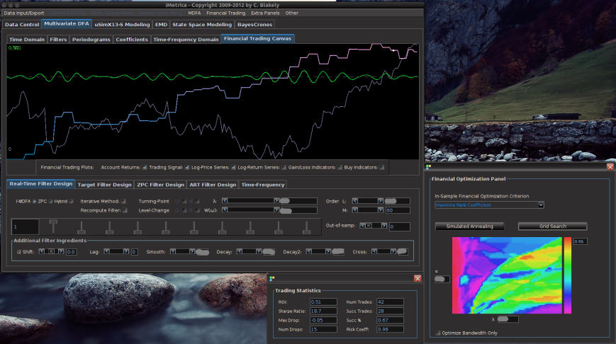The smoothness parameter is found on the Real-Time Filter Design interface in the sliding scrollbar marked $W(\omega)$ (see Figure 2) and in the sliding scrollbar marked $\alpha$ in the ZPC Filter Design panel (see Figure 4).

Quantization of information. In this sense, the quantization of information relates to how much past information is used to construct the trading signal. In MDFA, it is controlled by the length of the filter $L$ and is found on the Real-Time Filter Design interface (see Figure 2). In theory, as the filter length $L$ gets larger. the more past information from the financial time series is used resulting in a better approximation of the targeted filter. However, as the saying goes, there’s no such thing as a free lunch: increasing the filter length adds more degrees of freedom, which then leads to the age-old problem of over-fitting. The result: increased nonsense at the most concurrent observation of the signal and chaos out-of-sample. Fortunately, we can relieve the problem of over-fitting by using regularization (see Secondary Parameters). The length of the filter is controlled in the sliding scrollbar marked Order- $L$ in the Real-Time Filter Design panel (Figure 2).

As you might have suspected, there exists a so-called “uncertainty principle” regarding the timeliness and smoothness of the signal. Namely, one cannot achieve a perfectly timely signal (zero phase error in the filter) while at the same time remaining certain that the timely signal estimate is free of unwanted “noise” (perfectly filtered data in the stop-band of the filter). The greater the timeliness (better phase error), the lesser the smoothness (suppression of unwanted high-frequency noise). A happy combination of these two parameters is always desired, and thankfully there exists in iMetrica an interface to optimize these two parameters to achieve a perfect balance given one’s financial trading priorities. There has been much to say on this real-time direct filter “uncertainty” principle, and the interested reader can seek the gory mathematical details in an original paper by the inventor and good friend and colleague Professor Marc Wildi here.

The Secondary Parameters

Regularization of filters is the act of projecting the filter space into a lower dimensional space,reducing the effective number of degrees of freedom. Recently introduced by Wildi in 2012 (see the Elements paper), regularization has three different members to adjust according to the preferences of the signal extraction problem at hand and the data. The regularization parameters are classified as secondary parameters and are found in the Additional Filter Ingredients section in the lower portion of the Real-Time Filter Design interface (Figure 2). The regularization parameters are described as follows.

Regularization: smoothness. Not to be confused with the smoothness parameter found in the primary list of parameters, this regularization technique serves to project the filter coefficients of the trading signal into an approximation space satisfying a smoothness requirement, namely that the finite differences of the coefficients up to a certain order defined by the smoothness parameter are kept relatively small. This ultimately has the effect that the parameters appear smoother as the smooth parameter increases. Furthermore, as the approximation space becomes more “regularized” according to the requirement that solutions have “smoother” solutions, the effective degrees of freedom decrease and chances of over-fitting will decrease as well. The direct consequences of applying this type of regularization on the signal output are typically quite subtle, and depends clearly on how much smoothness is being applied to the coefficients. Personally, I usually begin with this parameter for my regularization needs to decrease the number of effective degrees of freedom and improve out-of-sample performance.

Regularization: decay. Employing the decay parameter ensures that the coefficients of the filter decay to zero at a certain rate as the lag of the filter increases. In effect, it is another form of information quantization as the trading signal will tend to lessen the importance of past information as the decay increases. This rate is governed by two decay parameter and higher the value, the faster the values decrease to zero. The first decay parameter adjusts the strength of the decay. The second parameter adjusts for how fast the coefficients decay to zero. Usually, just a slight touch on the strength of the decay and then adjusting for the speed of the decay is the order in which to proceed for these parameters. As with the smoothing regularization, the number of effective degrees of freedom will (in most cases) decreases as the decay parameter decreases, which is a good thing (in most cases).

Regularization: cross correlation. Used for building trading signals with multivariate data only, this regularization effect groups the latitudinal structure of the multivariate time series more closely, resulting in more weighted estimate of the target filter using the target data frequency information. As the cross regularization parameter increases, the filter coefficients for each time series tend to converge towards each other. It should typically be used in a last effort to control for over-fitting and should only be used if the financial time series data is on the same scale and all highly correlated.

The Tertiary Parameters

Phase-delay customization. The phase-delay of the filter at frequency zero, defined by the instantaneous rate of change of a filter’s phase at frequency zero, characterizes important information related to the timeliness of the filter. One can directly ensure that the phase delay of the filter at frequency zero is zero by adding constraints to the filter coefficients at computation time. This is done by setting the clicking the $i2$ option in the Real-Time Filter Design interface. To go further, one can even set the phase delay to an fixed value other than zero using the $i2$ scrollbar in the Additional Filter Ingredients box. Setting this value to a certain value (between -20 and 20 in the scrollbar) ensures that the phase delay at zero of the filter reacts as anticipated. It’s use and benefit is still under investigation. In any case, one can seamlessly test how this constraint affects the trading signal output in their own trading strategies directly by visualizing its performance in-sample using the Financial Trading canvas.

Differencing weight. This option, found in the Real-Time Filter Design interface as the checkbox labeled “d” (Figure 2), multiplies the frequency information (periodogram or discrete Fourier transform (DFT)) of the financial data by the weighting function $f(\omega) = 1/(1 - \exp(i \omega)), \omega \in (0,\pi)$ , which is the reciprocal of the differencing operator in the frequency domain. Since the Financial Trading platform in iMetrica strictly uses log-return financial time series to build trading signals, the use of this weighting function is in a sense a frequency-based “de-differencing” of the differenced data. In many cases, using the differencing weight provides better timeliness properties for the filter and thus the trading signal.

In addition to these three levels of parameters used in building real-time trading signals, there is a collection of more exotic “parameterization” strategies that exist in the iMetica MDFA module for fine tuning and constructing boosting trading performance. However, these strategies require more time to develop, a bit of experimentation, and a keen eye for filtering. We will develop more information and tutorials about these advanced filtering techniques for constructing effective trading signals in iMetrica in future articles on this blog coming soon. For now, we just summarize their main ideas.

Advanced Filtering Parameters

Hybrid filtering. In hybrid filtering, the goal is to filter a target signal additionally by injecting it with another filter of a different type that was constructed using the same data, but different paradigm or set of parameters. One method of hybrid filtering that is readily available in the MDFA module entails constructing Zero-Pole Combination filters using the ZPC Filter Design interface (Figure 4) and injecting the filter into the filter constructed in the Real-Time Filter Design interface (Figure 2) (see Wildi ZPC for more information). The combination (or hybrid) filter can then be accessed using one of the check box buttons in the filter interface and then adjusted using all the various levels of parameters above, and then used in the financial trading interface. The effect of this hybrid construction is to essentially improve either the smoothness or timeliness of any computed trading signal, while at the same time not succumbing to the nasty side-effects of over-fitting.

Forecasting and Smoothing signals. Smoothing signals in time series, as its name implies, involves obtaining a smoother estimate of certain signal in the past. Since the real-time estimate of a signal value in the past involves using more recent values, the signal estimation becomes more symmetrical as past and future values at a point in the past are used to estimate the value of the signal. For example, if today is after market hours on Friday, we can obtain a better estimate of the targeted signal for Wednesday since we have information from Thursday and Friday. In the opposite manner, forecasting involves projecting a signal into the future. However, since the estimate becomes even more “anti-symmetric”, the estimate becomes more polluted with noise. How these smoothed and forecasted signals can be used for constructing buy/sell trading signals in real-time is still purely experimental. With iMetrica, building and testing strategies that improve trading performance using either smoothed and forecasted signals (or both), is available.To produce either a smoothed or forecasted signal, there is a lag scrollbar available in the Real-Time Filter Design interface under Additional Filter Ingredients that enables one to compute either a smooth or forecasted signal. Setting the lag value $k$ in the scrollbar to any integer between -10 and 10 and the signal with the set lag applied is automatically computed. For negative lag values $k$ , the method produces a $k$ step-ahead forecast estimate of the signal. For positive values, the method produces a smoothed signal with a delay of $k$ observations.

Customized spectral weighting functions. In the spirit of customizing a trading signal to fit one’s priorities in financial trading, one also has the option of customizing the spectral density estimate of the data generating process to any design one wishes. In the computation of the real-time filter, the periodogram (or DFTs in multivariate case) is used as the default estimate of the spectral density weighting function. This spectral density weighting function in theory is supposed to serve as the spectrum of the underlying data generating process (DGP). However, since we have no possible idea about the underlying DGP of the price movement of publicly traded financial assets (other than it’s supposed to be pretty darn close to a random walk according to the Efficient Market Hypothesis), the periodogram is the best thing to an unbiased estimate a mortal human can get and is the default option in the MDFA module of iMetrica. However, customization of this weighting function is certainly possible through the use of the Target Filter Design interface. Not only can one design their target filter for the approximation of the concurrent filter, but the spectral density weighting function of the DGP can also be customized using some of the available options readily available in the interface. We will discuss these features in a soon-to-come discussion and tutorial on advanced real-time filtering methods.

Adaptive filtering. As perhaps the most advanced feature of the MDFA module, adaptive filtering is an elegant way to achieve building smarter filters based on previous filter realizations. With the goal of adaptive filtering being to improve certain properties of the output signal at each iteration without compensating with over-fitting, the adaptive process is of course highly nonlinear. In short, adaptive MDFA filtering is an iterative process in which a one begins with a desired filter, computes the output signal, and then uses the output signal as explanatory data in the next filtering round. At each iteration step, one has the freedom to change any properties of the filter that they desire, whether it be customization, regularization, adding negative lags, adding filter coefficient constraints, applying a ZPC filter, or even changing the pass-band in the target filter. The hope is to improve on certain properties of filter at each stage of the iterative process. An in-depth look at adaptive filtering and how to easily produce an adaptive filter using iMetrica is soon to come later this week.

Hybrid Signal Extraction, Machine Learning, and Algorithmic Financial Trading

Combining Computational Methodologies for Real-Time Learning and Signal Extraction

Tag Archives: filtering

High-Frequency Financial Trading with Multivariate Direct Filtering Part Deux: Index Futures

STOXX Europe 50 Index (STXE H3, Expiration March 18 2013)

S&P 500 Futures Index (ES H3, Expiration March 18 2013)

ASX Futures (YAPH3, Expiration March 18, 2013)

Conclusion

High-Frequency Financial Trading on FOREX with MDFA and R: An Example with the Japanese Yen

Example 2

Conclusion

The Frequency Effect: How to Infer Optimal Frequencies in Financial Trading

Hierarchy of Financial Trading Parameters