Realizing the Future with iMetrica and HEAVY Models

Posted on January 28, 2013 by Christian Dallas Blakely

In this article we steer away from multivariate direct filtering and signal extraction in financial trading and briefly indulge ourselves a bit in the world of analyzing high-frequency financial data, an always hot topic with the ever increasing availability of tick data in computationally convenient formats. Not only has high-frequency intraday data been the basis of higher frequency risk monitoring and forecasting, but it also provides access to building ‘smarter’ volatility prediction models using so-called realized measures of intraday volatility. These realized measures have been shown in numerous studies over the past 5 years or so to provide a solidly more robust indicator of daily volatility. While daily returns only capture close-to-close volatility, leaving much to be said about the actual volatility of the asset that was witnessed during the day, realized measures of volatility using higher frequency data such as second or minute data provide a much clearer picture of open-to-close variation in trading.

In this article, I briefly describe a new type of volatility model that takes into account these realized measures for volatility movement called High frEquency bAsed VolatilitY (HEAVY) models developed and pioneered by Shephard and Sheppard 2009. These models take as input both close-to-close daily returns $r_t$ as well as daily realized measures to yield better forecasting dynamics. The models have been shown to be endowed with the ability to not only track momentum in volatility, but also adjust for mean reversion effects as well as adjust quickly to structural breaks in the level of the volatility process. As the authors (Sheppard and Shephard, 2009) state in their original paper, the focus of these models is on predictive properties, rather than on non-parametric measurement of volatility. Furthermore, HEAVY models are much easier and more robust estimation wise than single source equations (GARCH, Stochastic Volatility) as they bring two sources of volatility information to identify a longer term component of volatility.

The goal of this article is three-fold. Firstly, I briefly review these HEAVY models and give some numerical examples of the model in action using a gnu-c library and Java package called heavy_model that I develped last year for the iMetrica software. The heavy_model package is available for download (either by this link or e-mail me) and features many options that are not available in the MATLAB code provided by Sheppard (bootstrapping methods, Bayesian estimation, track reparameterization, among others). I will then demonstrate the seamless ability to model volatility with these High frEquency bAsed VolatilitY models using iMetrica, where I also provide code for computing realized measures of volatility in Java with the help of an R package called highfrequency (Boudt, Cornelissen, and Payseur 2012).

HEAVY Model Definition

Let’s denote the daily returns as $r_1, r_2, \ldots, r_T$ , where $T$ is the total amount of days in the sample we are working with. In the HEAVY model, we supplement information to the daily returns by a so-called realized measure of intraday volatility based on higher frequency data, such as second, minute or hourly data. The measures are called daily realized measures and we will denote them as $RM_1, RM_2, \ldots, RM_T$ for the total number of days in the sample. We can think of these daily realized measures as an average of variance autocorrelations during a single day. They are supposed to provide a better snapshot of the ‘true’ volatility for a specific day $t$ . Although there are numerous ways of computing a realized measure, the easiest is the realized variance computed as $RM_t = \sum_j (X_{t+t_{j,t}} - X_{t+t_{j-1,t}})^2$ where $t_{j,t}$ are the normalized times of trades on day $t$ . Other methods for providing realized measures includes using Kernel based methods which we will discuss later in this article (see for example http://papers.ssrn.com/sol3/papers.cfm?abstract_id=927483).

Once the realized measures have been computed for $T$ days, the HEAVY model is given by:

$Var(r_t | \mathcal{F}_{t-1}^{HF}) = h_t = \omega_1 + \alpha RM_{t-1} + \beta h_{t-1} + \lambda r^2_t$

$E(RM_t | \mathcal{F}_{t-1}^{HF}) = \mu_t = \omega_2+ \alpha_R RM_{t-1} + \beta_R \mu_{t-1},$

where the stability constraints are $\alpha, \omega_1 \geq 0, \beta \in [0,1]$ and $\omega_2, \alpha_R \geq 0$ with $\lambda + \beta \in [0,1]$ and $\beta_R + \alpha_R \in [0,1]$ . Here, the $\mathcal{F}_{t-1}^{HF}$ denotes the high-frequency information from the previous day $t-1$ . The first equation models the close-to-close conditional variance and is akin to a GARCH type model, whereas the second equation models the conditional expectation of the open-to-close variation.

With the formulation above, one can easily see that slight variations to the model are perfectly plausible. For example, one could consider additional lags in either the realized measure $RM_t$ (akin to adding additional moving average parameters) or the conditional mean/variance variable (akin to adding autoregression parameters). One could also leave out the dependence on the squared returns $r^2_t$ by setting $\lambda$ to zero, which is what the original others recommended. A third variation is adding yet another equation to the pack that models a realized measure that takes into account negative and positive momentum to yield possibly better forecasts as it tracks both losses and gains in the model. In this case, one would add the third component by introducing a new equation for a realized semivariance to parametrically model statistical leverage eﬀects, where falls in asset prices are associated with increases in future volatility. With realized semivariance computed for the $T$ days as $RMS_1, \ldots RMS_T$ , the third equation becomes

$E(RMS_t | \mathcal{F}_{t-1}^{HF}) = \phi_t = \omega_3 + \alpha_{RS} RMS_{t-1} + \beta_{RS} \phi_{t-1}$

where $\alpha_{RS} + \beta_{RS} < 1$ and both positive.

HEAVY modeling in C and Java

To incorporate these HEAVY models into iMetrica, I began by writing a gnu-c library for providing a fast and efficient framework for both quasi-likelihood evaluation and a posteriori analysis of the models. The structure of estimating the models follows very closely to the original MATLAB code provided by Sheppard. However, in the c library I’ve added a few more useful tools for forecasting and distribution analysis. The Java code is essentially a wrapper for the c heavy_model library to provide a much cleaner approach to modeling and analyzing the HEAVY data such as the parameters and forecasts. While there are many ways to declare, implement, and analyze HEAVY models using the c/java toolkit I provide, the most basic steps involved are as follows.

heavyModel heavy = new heavyModel(); heavy.setForecastDimensions(n_forecasts, n_steps); heavy.setParameterValues(w1, w2, alpha, alpha_R, lambda, beta, beta_R); heavy.setTrackReparameter(0); heavy.setData(n_obs, n_series, series); heavy.estimateHeavyModel();

The first line declares a HEAVY model in java, while the second line sets the number of forecasts samples to compute and how many forecast steps to take. Forecasted values are provided for both the return variable $r_t$ (using a bootstrapping methodology) and the $h_t$ , $\mu_t$ variables. In the next line, the parameter values for the HEAVY model are initialized. These are the initial points that are utilized in the quasi-maximum likelihood optimization routine and can be set to any values that satisfy the model constraints. Here, $w1 = \omega_1, w2 = \omega_2$ .

The fourth line is completely optional and is used for toggling (0=off, 1=on) a reparameterization of the HEAVY model so the intercepts of both equations in the HEAVY model are explicitly related to the unconditional mean of squared returns $r^2$ and realized measures $RM_t$ . The reparameterization of the model has the advantage that it eliminates the estimation of $\omega_1, \omega_2$ and instead uses the unconditional means, leaving two less degrees of freedom in the optimization. See page 12 of the Shephard and Sheppard 2009 paper for a detailed explanation of the reparameterization. After setting the initial values, the data is set for the model by inputting the total number of observation $T$ , the number of series (normally set to 2 and the data in column-wise format (namely a double array of length n_obs x n_series, where the first column is the return data $r_t$ and the second column is the daily realized measure data. Finally, with the data set and the parameters initialized we estimate the model in the 6th line. Once the model is finished estimating (should take a few seconds, depending on the number of observations), the heavyModel java object stores the parameter values, forecasts, model residuals, likelihood values, and more. For example, one can print out the estimated model parameters and plot the forecasts of $h_t$ using the following:

heavy.printModelParameters(); heavy.plotForecasts(); Output: w_1 = 0.063 w_2 = 0.053 beta = 0.855 beta_R = 0.566 alpha = 0.024 alpha_R = 0.375 lambda = 0.087

Figure 1 shows the plot of the filtered $h_t, \mu_t$ values for 300 trading days from June 2011 to June 2012 of AAPL with the final 20 points being the forecasted values. Notice that the multistep ahead forecast shows momentum which is one of the attractive characteristics of the HEAVY models as mentioned in the original paper by Shephard and Sheppard.

Figure 1: Plots of the filtered returns and realized measures with 20 step forecasts for Verizon for 300 trading days.

We can also easily plot the estimated joint distribution function $F_{\zeta, \eta}$ by simply using the ﬁltered $h_t, \mu_t$ and computing the devolatilized values $\zeta_t = r_t/ \sqrt{h_t}$ , $\eta_t = (RM_t/\mu_t)^{1/2}$ , leading to the innovations for the model for $t = 2,\ldots,T$ .

Figure 2 below shows the empirical distribution of $F_{\zeta, \eta}$ for 600 days (nearly two years of daily observations from AAPL). The $\zeta_t$ sequence should be roughly a martingale diﬀerence sequences with unit variance and the $\eta_t$ sequence should have unit conditional means and of course be uncorrelated. The empirical results validate the theoretical values.

Figure 2: Scatter plot of the empirical distribution of devolatilized values for h and mu.

In order to compile and run the heavy_model library and the accompanying java wrapper, one must first be sure to meet the requirements for installation. The programs were extensively tested on a 64bit Linux machine running Ubuntu 12.04. The heavy_model library written in c uses the GNU Scientific Library (GSL) for the matrix-vector routines along with a statistical package in gnu-c called apophenia (Klemens, 2012) for the optimization routine. I’ve also included a wrapper for the GSL library called multimin.c which enables using the optimization routines from the GSL library, but were not heavily tested. The first version (version 00) of the heavy_model library and java wrapper can be downloaded at sourceforge.net/projects/highfrequency. As a precautionary warning, I must confess that none of the files are heavily commented in any way as this is still a project in progress. Improvements in code, efficiency, and documentation will be continuously coming.

After downloading the .tar.gz package, first ensure that GSL and Apophenia are properly installed and the libraries are correctly installed to the appropriate path for your gnu c compiler. Second, to compile the .c code, copy the makefile.test file to Makefile and then type make. To compile the heavyModel library and utilize the java heavyModel wrapper (recommended), copy makefile.lib to Makefile, then type make. After it constructs the libheavy.so, compile the heavyModel.java file by typing javac heavyModel.java. Note that the java files were complied successfully using the Oracle Java 7 SDK. If you have any questions about this or any of the c or java files, feel free to contact me. All the files were written by me (except for the optional multimin.c/h files for the optimization) and some of the subroutines (such as the HEAVY model simulation) are based on the MATLAB code by Sheppard. Even though I fully tested and reproduced the results found in other experiments exploring HEAVY models, there still could be bugs in the code. I have not fully tested every aspect (especially the Bayesian estimation components, an ongoing effort) and if anyone would like to add, edit, test, or comment on any of the routines involved in either the c or java code, I’d be more than happy to welcome it.

HEAVY Modeling in iMetrica

The Java wrapper to the gnu-c heavy_model library was installed in the iMetrica software package and can be used for GUI style modeling of high-frequency volatility. The HEAVY modeling environment is a feature of the BayesCronos module in iMetrica that also features other stochastic models for capturing and forecasting volatility such as (E)GARCH, stochastic volatility, mutlivariate stohastic factor modeling, and ARIMA modeling, all using either standard (Q)MLE model estimation or a Bayesian estimation interface (with histograms showing the MCMC results of the parameter chains).

Modeling volatility with HEAVY models is done by first uploading the data into the BayesCronos module (shown in Figure 3) through the use of either the BayesCronos Menu (featured on the top panel) or by using the Data Control Panel (see my previous article on Data Control).

Figure 3: BayesCronos interface in iMetrica for HEAVY modeling.

In the BayesCronos control panel shown above, we estimate a HEAVY model for the uploaded data (600 observations of $r_t, RM_t$ ) that were simulated from a model with omega_1 = 0.05, omega_2 = 0.10, beta = 0.8 beta_R = 0.3, alpha = 0.02, alpha_R = 0.3 (the simulation was done in the Data Control Module).

The model type is selected in the panel under the Model combobox. The number of forecasting steps and forecasting samples (for the $r_t$ variable) are selected in the Forecasting panel. Once those values are set, the model estimates are computed by pressing the “MLE” button in the bottom lower left corner. After the computing is done, all the available plots to analyze the HEAVY model are available by simply clicking the appropriate plotting checkboxes directly below the plotting canvas. This includes up to 5 forecasts, the original data, the filtered $h_t, \mu_t$ values, the residuals/empirical distributions of the returns and realized measures, and the pointwise likelihood evaluations for each observation. To see the estimated parameter values, simply click the “Parameter Values” button in the “Model and Parameters” panel and pop-up control panel will appear showing the estimated values for all the parameters.

Realized Measures in iMetrica

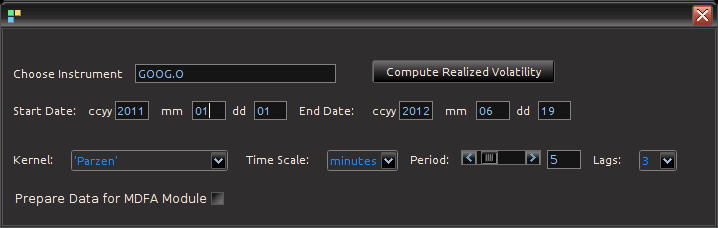
Figure 4: Computing Realized measures in iMetrica using a convenient realized measure control panel.

Importing and computing realized volatility measures in iMetrica is accomplished by using the control panel shown in Figure 4. With access to high frequency data, one simply types in the ticker symbol in the “Choose Instrument” box, sets the starting and ending date in the standard CCYY-MM-DD format, and then selects the kernel used for assembling the intraday measurements. The Time Scale sets the frequency of the data (seconds, minutes hours) and the period scrollbar sets the alignment of the data. The Lags combo box determines the bandwidth of the kernel measuring the volatility. Once all the options have been set, clicking on the “Compute Realized Volatility” button will then produce three data sets for the time period given between start date and end data: 1) The daily log-returns of the asset $r_1, \ldots, r_T$ 2) The log-price of the asset, and 3) The realized volatility measure $RM_1, \ldots, RM_T$ . Once the Java-R highfrequency routine has finished computing the realized measures, the data sets are automatically available in the Data Control Module of iMetrica. From here, one can annualize the realized measures using the weight adjustments in the Data Control Module (see Figure 5). Once content with the weighting, the data can then be exported to the MDFA module or the BayesCronos module for estimating and forecasting the volatility of GOOG using HEAVY models.

Figure 4: The log-return data (blue) and the (annualized) realized measure data using 5 minute returns (pink).

Figure 5: The log-return data (blue) and the (annualized) realized measure data using 5 minute returns (pink) for Google from 1-1-2011 to 6-19-2012.

The Realized Measure uploading in iMetrica utilizes a fantastic R package for studying and working with high frequency financial data called highfrequency (Boudt, Cornelissen, and Payseur 2012). To handle the analysis of high frequency financial data in java, I began by writing a Java wrapper to the R functions of the highfrequency R package to enable GUI interaction shown above in order to download the data into java and then iMetrica. The java environment uses library called RCaller that opens a live R kernel in the Java runtime environment from which I can call and R routines and directly load the data into Java. The initializing sequence looks like this.

caller.getRCode().addRCode("require (Runiversal)"); caller.getRCode().addRCode("require (FinancialInstrument)"); caller.getRCode().addRCode("require (highfrequency)"); caller.getRCode().addRCode("loadInstruments('/HighFreqDataDirectoryHere/Market/instruments.rda')"); caller.getRCode().addRCode("setSymbolLookup.FI('/HighFreqDataDirectoryHere/Market/sec',use_identifier='X.RIC',extension='RData')");
Here, I’m declaring the R packages that I will be using (first three lines) and then I declare where my HighFrequency financial data symbol lookup directory is on my computer (next two lines). This
then enables me to extract high frequency tick data directly into Java. After loading in the desired intrument ticker symbol names, I then proceed to extract the daily log-returns for the given time frame, and then compute the realized measures of each asset using the rKernelCov function in highfrequency R package. This looks something like
for(i=0;i<n_assets;i++) { String mark = instrum[i] + "<-" + instrum[i] + "['T09:30/T16:00',]";

caller.getRCode().addRCode(mark);

String rv = "rv"+i+"<-rKernelCov("+instrum[i]+"$Trade.Price,kernel.type ="+kernels[kern]+", kernel.param="+lags+",kernel.dofadj = FALSE, align.by ="+frequency[freq]+", align.period="+period+", cts=TRUE, makeReturns=TRUE)"

caller.getRCode().addRCode(rv);

caller.getRCode().addRCode("names(rv"+i+")<-'rv"+i+"'"); rvs[i] = "rv_list"+i;

caller.getRCode().addRCode("rv_list"+i+"<-lapply(as.list(rv"+i+"), coredata)"); }

In the first line, I’m looping through all the asset symbols (I create Java strings to load into the RCaller as commands). The second line effectively retrieves the data during market hours only (America/New_York time), then creates a string to call the rKernelCov function in R. I give it all the user defined parameters defined by strings as well. Finally, in the last two lines, I extract the results and put them into an R list from which the java runtime environment will read.

Conclusion

In this article I discussed a recently introduced high frequency based volatility model by Shephard and Sheppard and gave an introduction to three different high-performance tools beyond MATLAB and R that I’ve developed for analyzing these new stochastic models. The heavyModel c/java package that I made available for download gives a workable start for experimenting in a fast and efficient framework the benefit of using high frequency financial data and most notably realized measures of volatility to produce better forecasts. The package will continuously be updated for improvements in both documentation, bug fixes, and overall presentation. Finally, the use of the R package highfrequency embedded in java and then utilized in iMetrica gives a fully GUI experience to stochastic modeling of high frequency financial data that is both conveniently easy to use and fast.

Happy Extracting and Volatilitizing!

Building a Multi-Bandpass Financial Portfolio

Posted on January 16, 2013 by Christian Dallas Blakely

Animation 1: The changing periodogram for different in-sample sizes and selecting an appropriate band-pass component to the multi-bandpass filter.

Animation 1: Click the image to view the animation. The changing periodogram for different in-sample sizes and selecting an appropriate band-pass component to the multi-bandpass filter.

In my previous article, the third installment of the Frequency Effect trilogy, I introduced the multi-bandpass (MBP) filter design as a practical device for the extraction of signals in financial data that can be used for trading in multiple types of market environments. As depicted through various examples using daily log-returns of Google (GOOG) as my trading platform, the MBP demonstrated a promising ability to tackle the issue of combining both lowpass filters to include a local bias and slow moving trend while at the same time providing access to higher trading frequencies for systematic trading during sideways and volatile market trajectories. I identified four different types of market environments and showed through three different examples how one can attempt to pinpoint and trade optimally in these different environments.

After reading a well-written and informative critique of my latest article, I became motivated to continue along on the MBP bandwagon by extending the exploration of engineering robust trading signals using the new design. In Marc’s words (the reviewer) regarding the initial results of this latest design in MDFA signal extraction for financial trading : “I tend to believe that some of the results are not necessarily systematic and that some of the results – Chris’ preference – does not match my own priority. I understand that comparisons across various designs of the triptic may require a fixed empirical framework (Google/Apple on a fixed time span). But this restricted setting does not allow for more general inference (on other assets and time spans). And some of the critical trades are (at least in my perspective) close to luck.”

As my empirical framework was fixed in that I applied the designed filters to only one asset throughout the study and for a fixed time span of a year worth of in-sample data applied to 90 days out-of-sample, results showing the MBP framework applied to other assets and time frames might have made my presentation of this new design more convincing. Taking this relevant issue of limited empirical framework into account, I am extending my previous article many steps further by presenting in this article the creation of a collection of financial trading signals based entirely on the MBP filter. The purpose of this article is to further solidify the potential for MBP filters and extend applications of the new design to constructing signals for various types of financial assets and in-sample/out-of-sample time frames. To do this I will create a portfolio of assets comprised of a group of well known companies coupled with two commodity ETFs (exchange traded funds) and apply the MBP filter strategy to each of the assets using various out-of-sample time horizons. Consequently, this will generate a portfolio of trading signals that I can track over the next several months.

Portfolio selection

In choosing the assets for my portfolio, I arranged a group of companies/commodities whose products or services I use on a consistent basis (as arbitrary as any other portfolio selection method, right?). To this end, I chose Verizon (VZ) (service provider for my iPhone5), Microsoft (MSFT) (even though I mostly use Linux for my computing needs), Toyota (TM) ( I drive a Camry), Coffee (JO) (my morning espresso keeps the wheels turning), and Gold (GLD) (who doesn’t like Gold, a great hedge to any currency). For each of these assets, I built a trading signal using various in-sample time periods beginning summer of 2011 and ending toward the end of summer 2012, to ensure all seasonal market effects were included. The out-of-sample time period in which I test the performance of the filter for each asset ranges anywhere from 90 days to 125 days out-of-sample. I tried to keep the selection of in-sample and out-of-sample points as arbitrary as possible.

Portfolio Performance

And so here we go. The performance of the portfolio.

Coffee (NYSEARCA:JO)

Regularization: smooth = .22, decay = .22, decay2 = .02, cross = 0
MBP = [0, .2], [.44,.55]
Out-of-sample performance: 32 percent ROI in 110 days

In order to work with commodities in this portfolio, the easiest way is through the use of ETFs that are traded in open markets just as any other asset. I chose the Dow Jones-UBS Coffee Subindex JO which is intended to reflect the returns that are potentially available through an unleveraged investment in one futures contract on the commodity of coffee as well as the rate of interest that could be earned on cash collateral invested in specified Treasury Bills. To create the MBP filter for the JO index, I used JO and USO (a US Oil ETF) as the explanatory series from the dates of 5-5-2011 until 1-13-2013 (just a random date I picked from mid 2011, cinqo de mayo) and set the initial low-pass portion for the trend component of the MBP filter to [0, .17]. After a significant amount of regularization was applied, I added a bandpass portion to the filter by initializing an interval at [.4, .5]. 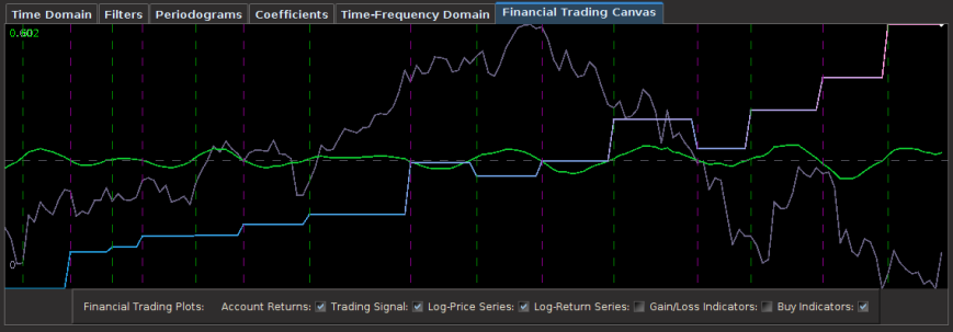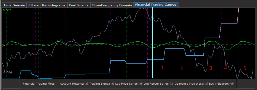This corresponded to the principal spectral peak in the periodogram which was located just below $\pi/6$ for the coffee fund. After setting the number of out-of-sample observations to 110, I then proceeded to optimize the regularization parameters in-sample while ensuring that the transfer functions of the filter were no greater than 1 at any point in the frequency domain. The result of the filter is plotted below in Figure 1, with the transfer functions of the filters plotted below it. The resulting trading signal from the MBP filter is in green and the out-of-sample portion after the cyan line, with the cumulative return on investment (ROI) percentage in blue-pink and the daily price of JO the coffee fund in gray.

Figure : The MBP filter for JO applied 110 Out-of-sample points (after cyan line).

Figure 1: The MBP filter for JO applied 110 Out-of-sample points (after cyan line).

Figure : Transfer function for the JO and USO MBP filters.

Figure 2: Transfer function for the JO and USO MBP filters.

Notice the out-of-sample portion of 110 observations behaving akin to the in-sample portion before it, with a .97 rank coefficient of the cumulative ROI resulting from the trades. The ROI in the out-of-sample portion was 32 percent total and suffered only 4 small losses out of 18 trades. The concurrent transfer functions of the MBP filter clearly indicate where the principal spectral peak for JO (blue-ish line) is directly under the bandpass portion of the filter. Notice the signal produced no trades during the steepest descent and rise in the price of coffee, while pinpointing precisely at the right moment the major turning point (right after the in-sample period). This is exactly what you would like the MBP signal to achieve.

Gold (SPDR Gold Trust, NYSEARCA:GLD)

As one of the more difficult assets to form a well-performing signal both in-sample and out-of-sample using the MBP filter, the GLD (NYSEARCA:GLD) ETF proved to be quite cumbersome in not only locating an optimal bandpass portion to the MBP, but also finding a relevant explaining series for GLD. In the following formulation, I settled upon using a US dollar index given by the PowerShares ETF UUP (NYSEARCA:UUP), as it ended up giving me a very linear performance that is consistent both in-sample and out-of-sample. The parameterization for this filter is given as follows:

Regularization: smooth = .22, decay = .22, decay2 = .02, cross = 0
MBP = [0, .2], [.44,.55]
Out-of-sample performance: 11 percent ROI in 102 days

Figure : Out-of-sample results of the MBP applied to the GLD ETF for 102 observations

Figure 3 : Out-of-sample results of the MBP applied to the GLD ETF for 102 observations

Figure : The Transfer Functions for the GLD and DIG filter.

Figure 4 : The Transfer Functions for the GLD and DIG filter.

Figure : Coefficients for the GLD and DIG filters. Each are of length 76.

Figure 5: Coefficients for the GLD and DIG filters. Each are of length 76.

The smoothness and decay in the coefficients is quite noticeable along with a slight lag correlation along the middle of the coefficients between lags 10 and 38. This trio of characteristics in the above three plots is exactly what one strives for in building financial trading signals. 1) The smoothness and decay of the coefficients, 2) the transfer functions of the filter not exceeding 1 in the low and band pass, and 3) linear performance both in-sample and out-of-sample of the trading signal.

Verizon (NYSE:VZ)

Regularization: smooth = .22, decay = 0, decay2 = 0, cross = .24
MBP = [0, .17], [.58,.68]
Out-of-sample performance: 44 percent ROI in 124 days trading

The experience of engineering a trading signal for Verizon was one of the longest and more difficult experiences out of the 5 assets in this portfolio. Strangely a very difficult asset to work with. Nevertheless, I was determined to find something that worked. To begin, I ended up using AAPL as my explanatory series (which isn’t a far fetched idea I would imagine. After all, I utilize Verizon as my carrier service for my iPhone 5). After playing around with the regularization parameters in-sample, I chose a 124 day out-of-day horizon for my Verizon to apply the filter to and test the performance. Surprisingly, the cross regularization seemed to produce very good results both out-of-sample. This was the only asset in the portfolio that required a significant amount of cross regularization, with the parameter touching the vicinity of .24. Another surprise was how high the timeliness parameter $\lambda$ was (40) in order to produce good in-sample and out-of-sample trading results. By far the highest amount of the 5 assets in this study. The amount of smoothing from the weighting function $W(\omega; \alpha)$ was also relatively high, reaching a value of 20.

The out-of-sample performance is shown in Figure 6. Notice how dampened the values of the trading signal are in this example, where the local bias during the long upswings is present, but not visible due to the size of the plot. The out-of-sample performance (after the cyan line) seems to be superior to that of the in-sample portion. This is most likely due to the fact that the majority of the frequencies that we were interested in, near $\pi/6$ , failed to become prominent in the data until the out-of-sample portion (there were around 120 trading days not shown in the plot as I only keep a maximum of 250 plotted on the canvas). With 124 out-of-sample observations, the signal produced a performance of 44 percent ROI. The filter seems to cleanly and consistently pick out local turning points, although not always at their optimal point, but the performance is quite linear, which is exactly what you strive for.

Figure : The out-of-sample performance on 124 observations from 7-2012 to 1-13-2013.

Figure 6: The out-of-sample performance on 124 observations from 7-2012 to 1-13-2013.

Figure : Coefficients of lag up to 76 of the Verizon-Apple filter,

Figure 7: Coefficients of lag up to 76 of the Verizon-Apple filter,

In the coefficients for the VZ and AAPL data shown in Figure 7, one can clearly see the distinguishing effects of the cross regularization along with the smooth regularization. Note that no decay regularization was needed in this example, with the resulting number of effective degrees of freedom in the construction of this filter being 48.2 an important number to consider when applying regularization to filter coefficients (filter length was 76),

Microsoft (NASDAQ:MSFT)

Regularization: smooth = .42, decay = .24, decay2 = .15, cross = 0
MBP = [0, .2], [.59,.72]
Out-of-sample performance: 31 percent ROI in 90 days trading

In the Microsoft data I used a time span of a year and three months for my in-sample period and a 90 day out-of-sample period from August through 1-13-2012. My explanatory series was GOOG (the search engine Bing and Google seem to have quite the competition going on, so why not) which seemed to correlate rather cleanly with the share price of MSFT. The first step in obtaining a bandpass after setting my lowpass filter to [0, .2] was to locate the principal spectral peak (shown in the periodogram figure below). I then adjusted the width until I had near monotone performance in-sample. Once the customization and regularization parameters were found, I applied the MSFT/AAPL filter to the 90 day out-of-sample period and the result is shown below. Notice that the effect of the local bias and slow moving trends from the lowpass filter are seen in the output trading signal (green) and help in identifying the long down swings found in the share price. During the long down swings, there are no trades due to the local bias from frequency zero.

Figure : Microsoft trading signal for 90 out-of-sample observations. The ROI out-of-sample is 31 percent.

Figure 8: Microsoft trading signal for 90 out-of-sample observations. The ROI out-of-sample is 31 percent.

Figure : Aggregate periodogram of MSFT and Google showing the principal spectral peak directly inside the bandpass.

Figure 9: Aggregate periodogram of MSFT and Google showing the principal spectral peak directly inside the bandpass.

Figure : The coefficients for the MSFT and GOOG series up to lag 76.

Figure 10: The coefficients for the MSFT and GOOG series up to lag 76.

With a healthy amount of regularization applied to the coefficient space, we can clearly see the smoothness and decay towards the end of the coefficient lags. The cross regularization parameter provided no improvement to either in-sample or out-of-sample performance and was left set to 0.

Despite the superb performance of the signal out-of-sample with a 31 percent ROI in 90 days in a period which saw the share price descend by 10 percent, and relatively smooth decaying coefficients with consistent performance both in and out-of-sample, I still feel like I could improve on these results with a better explanatory series than AAPL. That is one area of this methodology in which I struggle, namely finding “good” explanatory series to better fortify the in-sample metric space and produce more even more anticipation in the signals. At this point it’s a game of trial and error. I suppose I should find a good market economist to direct these questions to.

Toyota (NYSE:TM)

Regularization: smooth = .90, decay = .14, decay2 = .72, cross = 0
MBP = [0, .21], [.49,.67]
Out-of-sample performance: 21 percent ROI in 85 days trading

For the Toyota series, I figured my first explanatory series to test things with would be an asset pertaining to the price of oil. So I decided to dig up some research and found that DIG ( NYSEARCA:DIG), a ProShares ETF, provides direct exposure to the global price of oil and gas (in fact it is leveraged so it corresponds to twice the daily performance of the Dow Jones U.S. Oil & Gas Index). The out-of-sample performance, with heavy regularization in both smooth and decay, seems to perform quite consistently with in-sample, The signal shows signs of patience during volatile upswings, which is a sign that the local bias and slow moving trend extraction is quietly at work. Otherwise, the gains are consistent with just a few very small losses. At the end of the out-of-sample portion, namely the past several weeks since Black Friday (November 23rd), notice the quick climb in stock price of Toyota. The signal is easily able to deduce this fast climb and is now showing signs of slowdown from the recent rise (the signal is approaching the zero crossing, that’s how I know). I love what you do for me, Toyota! (If you were living in the US in the1990s, you’ll understand what I’m referring to).

Figure : Out-of-sample performance of the Toyota trading signal on 85 trading days.

Figure 11: Out-of-sample performance of the Toyota trading signal on 85 trading days.

Figure : Coefficients for the TM and DIG log-return series.

Figure 12: Coefficients for the TM and DIG log-return series.

Figure : The transfer functions for the TM and DIG filter coefficients.

Figure 13: The transfer functions for the TM and DIG filter coefficients.

The coefficients for the TM and DIG series depicted in Figure 12 show the heavy amount of smooth and decay (and decay2) regularization, a trio of parameters that was not easy to pinpoint at first without significant leakage above one in the filter transfer functions (shown in Figure 13). One can see that two major spectral peaks are present under the lowpass portion and another large one in the bandpass portion that accounts for the more frequent trades.

Conclusion

With these trading signals constructed for these five assets, I imagine I have a small but somewhat diverse portfolio, ranging from tech and auto to two popular commodities. I’ll be tracking the performance of these trading signals together combined as a portfolio over the next few months and continuously give updates. As the in-sample periods for the construction of these filters ended around the end of last summer and were already applied to out-of-sample periods ranging from 90 days to 124 (roughly one half to one third of the original in-sample period), with the significant amount of regularization applied, I am quite optimistic that the out-of-sample performance will continue to be the same over the next few months, but of course one can never be too sure of anything when it comes to market behavior. In the worse case scenario, I can always look into digging though my dynamic adaptive filtering and signal extraction toolkit.

Some general comments as I conclude this article. What I truly enjoy about these trading signals constructed for this portfolio experiment (and robust trading signals in general per my other articles on financial trading) is that when any losses out-of-sample or even in-sample occur, they tend to be extremely small relative to the average size of the gains. That is the sign of a truly robust signal I suppose; that not only does it perform consistently both in-sample and out-of-sample, but also that when losses do arrive, they are quite small. One characteristic that I noticed in all robust and high performing trading signals that I tend to stick with is that no matter what type of extraction definition you are targeting (lowpass, bandpass, or MBP), when an erroneous trade is executed (leading to a loss), the signal will quickly correct itself to minimize the loss. This is why the losses in robust signals tend to be small (look at any of the 5 trading signals produced for the portfolio in this article). Of course, all these good trading signal characteristics are in addition to the filter characteristics (smooth, slightly decaying coefficients with minimal effective degrees of freedom, transfer functions less than or equal to one everywhere, etc.)

Overall, although I’m quite inspired and optimistic with these results. there is still slight room for improvement in building these MBP filters, especially for low volatility sideways markets (for example, the one occurring in the Toyota stock price in the middle of the plot in Figure 11). In general, this is a difficult type of stock price movement in which any type of signal will have success. With low volatility and no trending movements, the log-returns are basically white noise – there is no pertinent information to extract. The markets are currently efficient and there is nothing you can do about it. Only good luck will win (in that case you’re as well off building a signal based on a coin flip). Typically the best you can do in these types of areas is prevent trading altogether with some sort of threshold on the signal, which is an idea I’ve had in my mind recently but haven’t implemented, or make sure any losses are small, which is exactly what my signal achieved in Figure 11 (and which is what any robust signal should do in the first place.)

Lastly, if you have a particular financial asset for which you would like to build a trading signal (similar to the examples shown above), I will be happy to take a stab at it using iMetrica (and/or give you pointers in the right direction if you would prefer to pursue the endeavor yourself). Just send me what asset you would like to trade on, and I’ll build the filter and send you the coefficients along with the parameters used. Offer holds for a limited time only!

Happy extracting.

The Frequency Effect Part III: Revelations of Multi-Bandpass Filters and Signal Extraction for Financial Trading

Posted on January 11, 2013 by Christian Dallas Blakely

Animation of the out-of-sample performance of one of the multibandpass filters built in this article for the daily returns of the price of Google. The resulting trading signal was extracted and yielded a trading performance near 39 percent ROI during an 80 day out-of-sample period on trading shares of Google.

To conclude the trilogy on this recent voyage through various variations on frequency domain configurations and optimizations in financial trading using MDFA and iMetrica, I venture into the world of what I call multi-bandpass filters that I recently implemented in iMetrica. The motivation of this latest endeavor in highlighting the fundamental importance of the spectral frequency domain in financial trading applications was wanting to gain better control of extracting signals and engineering different trading strategies through many different types of market movement in financial assets. There are typically four different basic types of movement a price pattern will take during its fractalesque voyage throughout the duration that an asset is traded on a financial market. These patterns/trajectories include

steady up-trends in share price
low volatility sideways patterns (close to white noise)
highly volatile sideways patterns (usually cyclical)
long downswings/trends in share price.

Using MDFA for signal extraction in financial time series, one typically indicates an a priori trading strategy through the design of the extractor, namely the target function $\Gamma(\omega)$ (see my previous two articles on The Frequency Effect). Designating a lowpass or bandpass filter in the frequency domain will give an indication of what kind of patterns the extracted trading signal will trade on. Traditionally one can set a lowpass with the goal of extracting trends (with the proper amount of timeliness prioritized in the parameterization), or one can opt for a bandpass to extract smaller cyclical events for more systematic trading during volatile periods. But now suppose we could have the best of both worlds at the same time. Namely, be profitable in both steady climbs and long tumbles, while at the same time systematically hacking our way through rough sideways volatile territory, making trades at specific frequencies embedded in the share price actions not found in long trends. The answer is through the construction of multi-band pass filters. Their construction is relatively simple, but as I will demonstrate in this article with many examples, they are a bit more difficult to pinpoint optimally (but it can be done, and the results are beautiful… both aesthetically and financially).

With the multi-bandpass defined as two separate bands given by $A := 1_{[\omega_0, \omega_1]}$ , $B := 1_{[\omega_2, \omega_3]}$ with $0 \leq \omega_0$ and $\omega_1 < \omega_2$ , zero everywhere else, it is easy to see that the motivation here is to seek a detection of both lower frequencies and low-mid frequencies in the data concurrently. With now up to four cutoff frequencies to choose from, this adds yet another few wrinkles in the degrees of freedom in parameterizing the MDFA setup. If choosing and optimizing one cutoff frequency for a simple low-pass filter in addition to customization and regularization parameters wasn’t enough, now imagine extracting signals with the addition of up to three more cutoff frequencies. Despite these additional degrees of freedom in frequency interval selection, I will later give a couple of useful hacks that I’ve found helpful to get one started down the right path toward successful extraction.

With this multi-bandpass definition for $\Gamma$ comes the responsibility to ensure that the customization of smoothness and timeliness is adjusted for the additional passband. The smoothing function $W(\omega; \alpha)$ for $\alpha \geq 0$ that acts on the periodogram (or discrete Fourier transforms in multivariate mode) is now defined piecewise according to the different intervals $[0,\omega_0]$ , $[\omega_1, \omega_2]$ , and $[\omega_3, \pi]$ . For example, $\alpha = 20$ gives a piecewise quadratic weighting function (an example shown in Figure 1) and for $\alpha = 10$ , the weighting function is piecewise linear. In practice, the piecewise power function smooths and rids of unwanted frequencies in the stop band much better than using a piecewise constant function. With these preliminaries defined, we now move on to the first steps in building and applying multiband pass filters.

Figure 1: Plot of the Piecewise Smoothing Function for alpha = 15 on a mutli-band pass filter.

To motivate this newly customized approach to building financial trading signals, I begin with a simple example where I build a trading signal for the daily share price of Google. We begin with a simple lowpass filter defined by $\Gamma(\omega) = 1$ if $\omega \in [0,.17]$ , and 0 otherwise. This formulation, as it includes the zero frequency, should provide a local bias as well as extract very slow moving trends. The trick with these filters for building consistent trading performance is ensure a proper grip on the timeliness characteristics of the filter in a very low and narrow filter passage. Regularization and smoothness using the weighting function shouldn’t be too much of a problem or priority as typically just only a small fraction of the available degrees of freedom on the frequency domain are being utilized, so not much concern for overfitting as long as you’re not using too long of a filter. In my example, I maxed out the timeliness $\lambda$ parameter and set the $\lambda_{smooth}$ regularization parameter to .3. Fortunately, no optimization of any parameter was needed in this example, as the performance was spiffy enough nearly right after gauging the timeliness parameter $\lambda$ . Figure 2 shows the resulting extracted trend trading signal in both the in-sample portion (left of the cyan colored line) and applied to 80 out-of-sample points (right of the cyan line, the most recent 80 daily returns of Google, namely 9-29-12 through today, 1-10-13). The blue-pink line shows the progression of the trading account, in return-on-investment percentage. The out-of-sample gains on the trades made were 22 percent ROI during the 80 day period.

Figure 1: The in-sample and out-of-sample gains made by constructing a low-pass filter employing a very high timeliness parameter and small amount of regularization in smoothness. The out-of-sample gains are nearly 30 percent and no losses on any trades.

Figure 2: The in-sample and out-of-sample gains made by constructing a low-pass filter employing a very high timeliness parameter and small amount of regularization in smoothness. The out-of-sample gains are nearly 30 percent and no losses on any trades.

Although not perfect, the trading signal produces a monotonic performance both in-sample and out-of-sample, which is exactly what you strive for when building these trend signals for trading. The performance out-of-sample is also highly consistent (in regards to trading frequency and no losses on any trades) with the in-sample performance. With only 4 trades being made, they were done at very interesting points in the trajectory of the Google share price. Firstly, notice that the local bias in the largest upswing is accounted for due to the inclusion of frequency zero in the low pass filter. This (positive) local bias continues out-of-sample until, interestingly enough, two days before one of the largest losses in the share price of Google over the past couple years. A slightly earlier exit out of this long position (optimally at the peak before the down turn a few days before) would have been more strategic; perhaps further tweaking of various parameters would have achieved this, but I happy with it for now. The long position resumes a few days after the dust settles from the major loss, and the local bias in the signal helps once again (after trade 2). The next few weeks sees shorter downtrending cyclical effects, and the signal fortunately turns positively increasingly right before another major turning point for an upswing in the share price. Finally, the third transaction ends the long position at another peak (3), perfect timing. The fourth transaction (no loss or gain) was quickly activated after the signal saw another upturn, and thus is now in the long position (hint: Google trending upward). 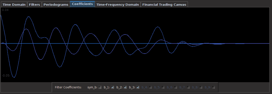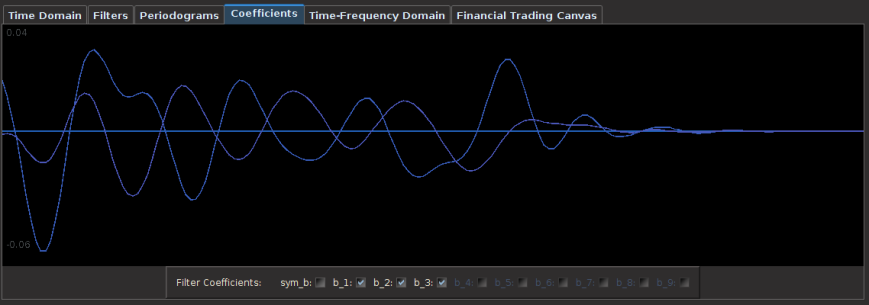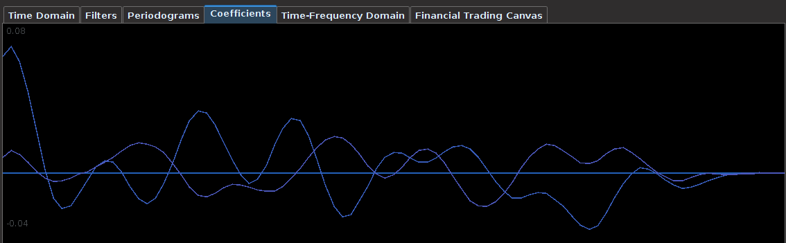Figure 3 shows the transfer functions $\hat{\Gamma}$ for both the sets of explanatory log-return data and Figure 4 depicts the coefficients for the filter. Notice that in the coefficients plot, much more weight is being assigned to past values of the log-return data with extreme (min and max values) at around lags 15 and 30 for the GOOG coefficients (blue-ish line). The coefficients are also quite smooth due to the slight amount of smooth regularization imposed.

Figure 3: Transfer functions for the concurrent trend filter applied to GOOG.

Figure 4: The filter coefficients for the log-return data.

Now suppose we wish to extract a trading signal that performs like a trend signal during long sweeping upswings or downswings, and at the same time shares the property that it extracts smaller cyclical swings during a sideways or highly volatile period. This type of signal would be endowed with the advantage that we could engage in a long position during upswings, trade systematically during sideways and volatile times, and on the same token avoid aggressive long-winded downturns in the price. Financial trading can’t get more optimistic then that, right? Here is where the magic of the multi-bandpass comes in. I give my general “how-to” guidelines in the following paragraphs as a step-by-step approach. As a forewarning, these signals are not easy to build, but with some clever optimization and patience they can be done.

In this new formulation, I envision not only being able to extract a local bias embedded in the log-return data but also gain information on other important frequencies to trade on while in sideways markets. To do this, I set up the lowpass filter as I did earlier on $[0,\omega_0]$ . The choice of $\omega_0$ is highly dependent on the data and should be located through a priori investigations (as I did above, without the additional bandpass).

Animation 2: Example of constructing a multiband pass using the Target Filter control panel in iMetrica. Initially, a low-pass filter is set, then the additional bandpass is added by clicking "Multi-Pass" checkbox. The location is then moved to the desired location using the scrollbars. The new filters are computed automaticall if "Auto" is checked on (lower left corner).

Click on the Animation 2: Example of constructing a multiband pass using the Target Filter control panel in iMetrica. Initially, a low-pass filter is set, then the additional bandpass is added by clicking “Multi-Pass” checkbox. The location is then moved to the desired location using the scrollbars. The new filters are computed automaticall if “Auto” is checked on (lower left corner).

Before setting any parameterization regarding customization, regularization, or filter constraints, I perform a quick scan of the periodogram (averaged periodogram if in multivariate mode) to locate what I call principal trading frequencies in the data. In the averaged periodogram, these frequencies are located at the largest spectral peaks, with the most useful ones for our purposes of financial trading typically before $\pi/4$ . The largest of these peaks will be defined from here on out as the principal spectral peak (PSP). Figure 6 shows an example of an averaged periodogram of the log-return for GOOG and AAPL with the PSP indicated. You might note that there exists a much larger spectral peak located at $7\pi/12$ , but no need to worry about that one (unless you really enjoy transaction costs). I locate this PSP as a starting point for where I want my signal to trade.

Figure 5: Principal spectral peak in the log-return data of GOOG and AAPL.

In the next step, I place a bandpass of width around .15 so that the PSP is dead-centered in the bandpass. Fortunately with iMetrica, this is a seamlessly simple task with just the use of a scrollbar to slide the positioning of this bandpass (and also adjust the lowpass) to where I desire. Animation 2 above (click on it to see the animation) shows this process of setting a multi-passband in the MDFA Target Filter control panel. Notice as I move the controls for the location of the bandpass, the filter is automatically recomputed and I can see the changes in the frequency response functions $\hat{\Gamma}$ instantaneously.

With the bandpass set along with the lowpass, we can now view how the in-sample performance is behaving at the initial configuration. Slightly tweaking the location of the bandpass might be necessary (width not so much, in my experience between .15 and .20 is sufficient). The next step in this approach is now to not only adjust for the location of the bandpass while keeping the PSP located somewhat centered, but also adding the effects of regularization to the filter as well. With this additional bandpass, the filter has a tendency to succumb to overfitting if one is not careful enough.

In my first filter construction attempt, I placed my bandpass at $[.49,.65]$ with the PSP directly under it. I then optimized the regularization controls in-sample (a feature I haven’t discussed yet) and slightly tweaked the timeliness parameter (ended up setting it to 3) and my result (drumroll…) is shown in Figure 6.

Figure 6: The trading performance and signal for the initial attempt at a building a multiband pass fitler.

Not bad for a first attempt. I was actually surprised at how few trades there were out-of-sample. Although there are no losses during the 80 days out-of-sample (after cyan line), and the signal is sort of what I had in mind a priori, the trades are minimal and not yielding any trading action during the period right after the large loss in Google when the market was going sideways and highly volatile. Notice that the trend signal gained from the lowpass filter indeed did its job by providing the local bias during the large upswing and then selling directly at the peak (first magenta dotted line after the cyan line). There are small transactions (gains) directly after this point, but still not enough during the sideways market after the drop. I needed to find a way to tweak the parameters and/or cutoff to include higher frequencies in the transactions.

In my second attempt, I kept the regularization parameters as they were but this time increased the bandpass to the interval $[.51, .68]$ , with the PSP still underneath the bandpass, but now catching on to a few more higher frequencies then before. I also slightly increased the length of the filter to see if that had any affect. After optimizing on the timeliness parameter $\lambda$ in-sample, I get a much improved signal. Figure 7 shows this second attempt.

Figure 7: The trading performance and signal for the second attempt at construction a multiband pass filter. This one included a few more higher frequencies.

Upon inspection, this signal behaves more consistently with what I had in mind. Notice that directly out-of-sample during the long upswing, the signal (barely) shows signs of the local bias, but enough not to make any trades fortunately. However, in this signal, we see that filter is much too late in detecting the huge loss posted by Google, and instead sells immediately after (still a profit however). Then during the volatile sideways market, we see more of what we were wishing for; timely trades to the earn the signal a quick 9 percent in the span of a couple weeks. Then the local bias kicks in again and we see not another trade posted during this short upswing, taking advantage of the local trend. This signal earned a near 22 percent ROI during the 80 day out-of-sample trading period, however not as good as the previous signal at 32 percent ROI.

Now my priority was to find another tweak that I could perform to change the trading structure even more. I’d like it to be even more sensitive to quick downturns, but at the same time keep intact the sideways trading from the signal in Figure 7. My immediate intuition was to turn on the i2 filter constraint and optimize the time-shift, similar to what I did in my previous article, part deux of the Frequency Effect. I also lessened the amount of smoothing from my weighting function $W(\omega; \alpha)$ , turned off any amount of decay regularization that I had and voila, my final result in Figure 8.

Figure 8: Third attempt at building a multiband pass filter. Here, I turn on i2 filter constraint and optimize the time shift.

While the consistency with the in-sample performance to out-of-sample performance is somewhat less than my previous attempts, out-of-sample performs nearly exactly how I envisioned. There are only two small losses of less than 1 percent each, and the timeliness of choosing when to sell at the tip of the peak in the share price of Google couldn’t have been better. There is systematic trading governed by the added multiband pass filter during the sideways and slight upswing toward the end. Some of the trades are made later than what would be optimal (the green lines enter a long position, magenta sells and enters short position), but for the most part, they are quite consistent. It’s also very quick in pinpointing its own erronous trades (namely no huge losses in-sample or out of sample). There you have it, a near monotonic performance out-of-sample with 39 percent ROI.

In examining the coefficients of this filter in Figure 9, we see characteristics of a trend filter as coefficients are largely weighting the middle lags much more than than initial or end lags (note that no decay regularization was added to this filter, only smoothness) . While at the same time however, the coefficients also weight the most recent log-return observations unlike the trend filter from Figure 4, in order to extract signals for the more volatile areas. The undulating patterns also assist in obtaining good performance in the cyclical regions.

Figure 9: The coefficients of the final filter depicting characteristics of both a trend and bandpass filter, as expected.

Finally, the frequency response functions of the concurrent filters show the effect of including the PSP in the bandpass (figure 10). Notice, the largest peak in the bandpass function is found directly at the frequency of the PSP, ahh the PSP. I need to study this frequency with more examples to get a more clear picture to what it means. In the meantime, this is the strategy that I would propose. If you have any questions about any of this, feel free to email me. Until next time, happy extracting!

Figure 10: The frequency response functions of the multiband filter.

Figure 10: The frequency response functions of the multi-bandpass filter.

The Frequency Effect Part Deux: Shifting Time at Frequency Zero For Better Trading Performance

Posted on January 3, 2013 by Christian Dallas Blakely

Animation 1: The out-of-sample performance over 60 trading days of signal built using a custom i2 criterion. With 5 trades and 4 successful, the ROI is nearly 40 percent.

Animation 1: The out-of-sample performance over 60 trading days of a signal built using an optimized time-shift criterion. With 5 trades and 4 successful, the ROI is nearly 40 percent over 3 month.

What is an optimized time-shift? Is it important to use when building successful financial trading signals? While the theoretical aspects of the frequency zero and vanishing time-shift can be discussed in a very formal and mathematical manner, I hope to answer these questions in a more simple (and applicable) way in this article. To do this, I will give an informative and illustrated real world example in this unforeseen continuation of my previous article on the frequency effect a few days ago. I discovered something quite interesting after I got an e-mail from Herr Doktor Marc (Wildi) that nudged me even further into my circus of investigations in carving out optimal frequency intervals for financial trading (see his blog for the exact email and response). So I thought about it and soon after I sent my response to Marc, I began to question a few things even further at 3am in the morning while sipping on some Asian raspberry white tea (my sleeping patterns lately have been as erratic as fiscal cliff negotiations), and came up with an idea. Firstly, there has to be a way to include information about the zero-frequency (this wasn’t included in my previous article on optimal frequency selection). Secondly, if I’m seeing promising results using a narrow band-pass approach after optimizing the location and distance, is there anyway to still incorporate the zero-frequency and maybe improve results even more with this additional frequency information?

Frequency zero is an important frequency in the world of nonstationary time series and model-based time series methodologies as it deals with the topic of unit roots, integrated processes, and (for multivariate data) cointegration. Fortunately for you (and me), I don’t need to dwell further into this mess of a topic that is cointegration since typically, the type of data we want to deal with in financial trading (log-returns) is closer to being stationary (namely close to being white noise, ehem, again, close, but not quite). Nonetheless, a typical sequence of log-return data over time is never zero-mean, and full of interesting turning points at certain frequency bands. In essence, we’d somehow like to take advantage of that and perhaps better locate local turning points intrinsic to the optimal trading frequency range we are dealing with.

The perfect way to do this is through the use of the time-shift value of the filter. The time-shift is defined by the derivative of the frequency response (or transfer) function at zero. Suppose we have an optimal bandpass set at $(\omega_0, \omega_1) \subset [0,\pi]$ where $\omega_0 > 0$ . We can introduce a constraint on the filter coefficients so as to impose a vanishing time-shift at frequency zero. As Wildi says on page 24 of the Elements paper: “A vanishing time-shift is highly desirable because turning-points in the filtered series are concomitant with turning-points in the original data.” In fact, we can take this a step further and even impose an arbitrary time-shift with the value $s$ at frequency zero, where $s$ is any real number. In this case, the derivative of the frequency response function (transfer function) $\hat{\Gamma}(\omega)$ at zero is $s$ . As explained on page 25 of Elements, this is implemented as $\frac{d}{d \omega} |_{\omega=0} \sum_{l=0}^{L-1} b_j \exp(-i j \omega) = s$ , which implies $b_1 + 2b_2 + \cdots + (L-1) b_{L-1} = s$ .

This constraint can be integrated into the MDFA formulation, but then of course adds another parameter to an already full-flight of parameters. Furthermore, the search for the optimal $s$ with respect to a given financial trading criterion is tricky and takes some hefty computational assistance by a robust (highly nonlinear) optimization routine, but it can be done. In iMetrica I’ve implemented a time-shift turning point optimizer, something that works well so far for my taste buds, but takes a large burden of computational time to find.

To illustrate this methodology in a real financial trading application, I return to the same example I used in my previous article, namely using daily log-returns of GOOG and AAPL from 6-3-2011 to 12-31-2012 to build a trading signal. This time to freshen things up a but, I’m going to target and trade shares of Apple Inc. instead of Google. Quickly, before I begin, I will swiftly go through the basic steps of building trading signals. If you’re already familiar, feel free to skip down two paragraphs.

As I’ve mentioned in the past, fundamentally the most important step to building a successful and robust trading signal is in choosing an appropriate preliminary in-sample metric space in which the filter coefficients for the signal are computed. This preliminary in-sample metric space represents by far the most critically important aspect of building a successful trading signal and is built using the following ingredients:

The target and explanatory series (i.e. minute, hourly, daily log-returns of financial assets)
The time span of in-sample observations (i.e. 6 hours, 20 days, 168 days, 3 years, etc.)

Choosing the appropriate preliminary in-sample metric space is beyond the scope of this article, but will certainly be discussed in a future article. Once this in-sample metric space has been chosen, one can then proceed by choosing the optimal extractor (the frequency bandpass interval) for the metric space. While concurrently selecting the optimal extractor, one must begin warping and bending the preliminary metric space through the use of the various customization and regularization tools (see my previous Frequency Effect article, as well as Marc’s Elements paper for an in-depth look at the mathematics of regularization and customization). These are the principle steps.

Now let’s look at an example. In the .gif animation at the top of this article, I featured a signal that I built using this time-shift optimizer and a frequency bandpass extractor heavily centered around the frequency $\pi/12$ , which is not a very frequent trading frequency, but has its benefits, as we’ll see. The preliminary metric space was constructed by an in-sample period using the daily log-returns of GOOG and AAPL and AAPL as my target is from 6-4-2011 to 9-25-2012, nearly 16 months of data. Thus we mention that the in-sample includes many important news events from Apple Inc. such as the announcement of the iPad mini, the iPhone 4S and 5, and the unfortunate sad passing of Steve Jobs. I then proceeded to bend the preliminary metric space with a heavy dosage of regularization, but only a tablespoon of customization¹. Finally, I set the time-shift constraint and applied my optimization routine in iMetrica to find the value $s$ that yields the best possible turning-point detector for the in-sample metric space. The result is shown in Figure 1 below in the slide-show. The in-sample signal from the last 12 months or so (no out-of-sample yet applied) is plotted in green, and since I have future data available (more than 60 trading days worth from 9-25 to present), I can also approximate the target symmetric filter (the theoretically optimal target signal) in order to compare things (a quite useful option available with the click of a button in iMetrica I might add). I do this so I can have a good barometer of over-fitting and concurrent filter robustness at the most recent in-sample observation. Figure 1 in the slide-show below, the trading signal is in green, the AAPL log-return data in red, and the approximated target signal in gray (recall that if you can approximate this target signal (in gray) arbitrarily well, you win, big).

: Figure 1: Trading signal with time-shift constraint set and optimized according to a financial trading criterion.

: Figure 2: Trading signal without the time-shift constraint set.

Notice that at the very endpoint (the most challenging point to achieve greatness) of the signal in Figure 1, the filter does a very fine job at getting extremely close. In fact, since the theoretical target signal is only a Fourier approximation of order 60, my concurrent signal that I built might even be closer to the ‘true value’, who knows. Achieving exact replication of the target signal (gray) elsewhere is a little less critical in my experience. All that really matters is that it is close in moving above and below zero to the targeted intention (the symmetric filter) and close at the most recent in-sample observation. Figure 2 above shows the signal without the time-shift constraint and optimization. You might be inclined to say that there is no real big difference. In fact, the signal with no time-shift constraint looks even better. It’s hard to make such a conclusion in-sample, but now here is where things get interesting.

We apply the filter to the out-of-sample data, namely the 60 tradings days. Figure 3 shows the out-of-sample performance over these past 60 trading days, roughly October, November, and December, (12-31-2012 was the latest trading day), of the signal without the time-shift constraint. Compare that to Figure 4 which depicts the performance with the constraint and optimization. Hard to tell a difference, but let’s look closer at the vertical lines. These lines can be easily plotted in iMetrica using the plot button below the canvas named Buy Indicators. The green line represents where the long position begins (we buy shares) and the exit of a short position. The magenta line represents where selling the shares occurs and the entering of a short position. These lines, in other words, are the turning point detection lines. They determine where one buys/sells (enter into a long/short position). Compare the two figures in the out-of-sample-portion after the light cyan line (indicated in Figure 4 but not Figure 3, sorry).

Figure 3: Out-of-sample performance of the signal built without time-shift constraint The out-of-sample period beings where the light cyan line is from Figure 4 below.

Figure 4: Out-of-sample performance of the signal built with time-shift constraint and optimized for turning point-detection, The out-of-sample period beings where the light cyan is.

Notice how the optimized time-shift constraint in the trading signal in Figure 4 pinpoints to a close perfection where the turning points are (specifically at points 3, 4,and 5). The local minimum turning point was detected exactly at 3, and nearly exact at 4 and 5. The only loss out of the 5 trades occurred at 2, but this was more the fault of the long unexpected fall in the share price of Apple in October. Fortunately we were able to make up for those losses (and then some) at the next trade exactly at the moment a big turning point came (3). Compare this to the non optimized time-shift constrained signal (Figure 3), and how the second and third turning points are a bit too late and too early, respectively. And remember, this performance is all out-of-sample, no adjustments to the filter have been made, nothing adaptive. To see even more clearly how the two signals compare, here are gains and losses of the 5 actual trades performed out-of-sample (all numbers are in percentage according to gains and losses in the trading account governed only by the signal. Positive number is a gain, negative a loss)

Without Time-Shift Optimization With Time-Shift Optimization

Trade 1: 29.1 -> 38.7 = 9.6 14.1 -> 22.3 = 8.2
Trade 2: 38.7 -> 32.0 = -6.7 22.3 -> 17.1 = -5.2
Trade 3: 32.0 -> 40.7 = 8.7 17.1 -> 30.5 = 13.4
Trade 4: 40.7 -> 48.2 = 7.5 30.5 -> 41.2 = 10.7
Trade 5: 48.2 -> 60.2 = 12.0 41.2 -> 53.2 = 12.0

The optimized time-shift signal is clearly better, with an ROI of nearly 40 percent in 3 months of trading. Compare this to roughly 30 percent ROI in the non-constrained signal. I’ll take the optimized time-shift constrained signal any day. I can sleep at night with this type of trading signal. Notice that this trading was applied over a period in which Apple Inc. lost nearly 20 percent of its share price.

Another nice aspect of this trading frequency interval that I used is that trading costs aren’t much of an issue since only 10 transactions (2 transaction each trade) were made in the span of 3 months, even though I did set them to be .01 percent for each transaction nonetheless.

To dig a bit deeper into plausible reasons as to why the optimization of the time-shift constraint matters (if only even just a little bit), let’s take a look at the plots of the coefficients of each respective filter. Figure 5 depicts the filter coefficients with the optimized time-shift constraint, and Figure 6 shows the coefficients without it. Notice how in the filter for the AAPL log-return data (blue-ish tinted line) the filter privileges the latest observation much more, while slowly modifying the others less. In the non optimized time-shift filter, the most recent observation has much less importance, and in fact, privileges a larger lag more. For timely turning point detection, this is (probably) not a good thing. Another interesting observation is that the optimized time-shift filter completely disregards the latest observation in the log-return data of GOOG (purplish-line) in order to determine the turning points. Maybe a “better” financial asset could be used for trading AAPL? Hmmm…. well in any case I’m quite ecstatic with these results so far. I just need to hack my way into writing a better time-shift optimization routine, it’s a bit slow at this point. Until next time, happy extracting. And feel free to contact me with any questions.

Figure 5: The filter coefficients with time-shift optimization.

Figure 6: The filter coefficients without the time-shift optimization.

¹ I won’t disclose quite yet how I found these optimal parameters and frequency interval or reveal what they are as I need to keep some sort of competitive advantage as I presently look for consulting opportunities 😉 .

Hybrid Signal Extraction, Machine Learning, and Algorithmic Financial Trading

Combining Computational Methodologies for Real-Time Learning and Signal Extraction

Monthly Archives: January 2013

Realizing the Future with iMetrica and HEAVY Models

HEAVY Model Definition

HEAVY modeling in C and Java

HEAVY Modeling in iMetrica

Realized Measures in iMetrica

Conclusion

Building a Multi-Bandpass Financial Portfolio

Portfolio selection

Portfolio Performance

Coffee (NYSEARCA:JO)

Gold (SPDR Gold Trust, NYSEARCA:GLD)

Verizon (NYSE:VZ)

Microsoft (NASDAQ:MSFT)

Toyota (NYSE:TM)

Conclusion

The Frequency Effect Part III: Revelations of Multi-Bandpass Filters and Signal Extraction for Financial Trading

The Frequency Effect Part Deux: Shifting Time at Frequency Zero For Better Trading Performance