Building a Multi-Bandpass Financial Portfolio

Posted on January 16, 2013 by Christian Dallas Blakely

Animation 1: The changing periodogram for different in-sample sizes and selecting an appropriate band-pass component to the multi-bandpass filter.

Animation 1: Click the image to view the animation. The changing periodogram for different in-sample sizes and selecting an appropriate band-pass component to the multi-bandpass filter.

In my previous article, the third installment of the Frequency Effect trilogy, I introduced the multi-bandpass (MBP) filter design as a practical device for the extraction of signals in financial data that can be used for trading in multiple types of market environments. As depicted through various examples using daily log-returns of Google (GOOG) as my trading platform, the MBP demonstrated a promising ability to tackle the issue of combining both lowpass filters to include a local bias and slow moving trend while at the same time providing access to higher trading frequencies for systematic trading during sideways and volatile market trajectories. I identified four different types of market environments and showed through three different examples how one can attempt to pinpoint and trade optimally in these different environments.

After reading a well-written and informative critique of my latest article, I became motivated to continue along on the MBP bandwagon by extending the exploration of engineering robust trading signals using the new design. In Marc’s words (the reviewer) regarding the initial results of this latest design in MDFA signal extraction for financial trading : “I tend to believe that some of the results are not necessarily systematic and that some of the results – Chris’ preference – does not match my own priority. I understand that comparisons across various designs of the triptic may require a fixed empirical framework (Google/Apple on a fixed time span). But this restricted setting does not allow for more general inference (on other assets and time spans). And some of the critical trades are (at least in my perspective) close to luck.”

As my empirical framework was fixed in that I applied the designed filters to only one asset throughout the study and for a fixed time span of a year worth of in-sample data applied to 90 days out-of-sample, results showing the MBP framework applied to other assets and time frames might have made my presentation of this new design more convincing. Taking this relevant issue of limited empirical framework into account, I am extending my previous article many steps further by presenting in this article the creation of a collection of financial trading signals based entirely on the MBP filter. The purpose of this article is to further solidify the potential for MBP filters and extend applications of the new design to constructing signals for various types of financial assets and in-sample/out-of-sample time frames. To do this I will create a portfolio of assets comprised of a group of well known companies coupled with two commodity ETFs (exchange traded funds) and apply the MBP filter strategy to each of the assets using various out-of-sample time horizons. Consequently, this will generate a portfolio of trading signals that I can track over the next several months.

Portfolio selection

In choosing the assets for my portfolio, I arranged a group of companies/commodities whose products or services I use on a consistent basis (as arbitrary as any other portfolio selection method, right?). To this end, I chose Verizon (VZ) (service provider for my iPhone5), Microsoft (MSFT) (even though I mostly use Linux for my computing needs), Toyota (TM) ( I drive a Camry), Coffee (JO) (my morning espresso keeps the wheels turning), and Gold (GLD) (who doesn’t like Gold, a great hedge to any currency). For each of these assets, I built a trading signal using various in-sample time periods beginning summer of 2011 and ending toward the end of summer 2012, to ensure all seasonal market effects were included. The out-of-sample time period in which I test the performance of the filter for each asset ranges anywhere from 90 days to 125 days out-of-sample. I tried to keep the selection of in-sample and out-of-sample points as arbitrary as possible.

Portfolio Performance

And so here we go. The performance of the portfolio.

Coffee (NYSEARCA:JO)

Regularization: smooth = .22, decay = .22, decay2 = .02, cross = 0
MBP = [0, .2], [.44,.55]
Out-of-sample performance: 32 percent ROI in 110 days

In order to work with commodities in this portfolio, the easiest way is through the use of ETFs that are traded in open markets just as any other asset. I chose the Dow Jones-UBS Coffee Subindex JO which is intended to reflect the returns that are potentially available through an unleveraged investment in one futures contract on the commodity of coffee as well as the rate of interest that could be earned on cash collateral invested in specified Treasury Bills. To create the MBP filter for the JO index, I used JO and USO (a US Oil ETF) as the explanatory series from the dates of 5-5-2011 until 1-13-2013 (just a random date I picked from mid 2011, cinqo de mayo) and set the initial low-pass portion for the trend component of the MBP filter to [0, .17]. After a significant amount of regularization was applied, I added a bandpass portion to the filter by initializing an interval at [.4, .5]. This corresponded to the principal spectral peak in the periodogram which was located just below $\pi/6$ for the coffee fund. After setting the number of out-of-sample observations to 110, I then proceeded to optimize the regularization parameters in-sample while ensuring that the transfer functions of the filter were no greater than 1 at any point in the frequency domain. The result of the filter is plotted below in Figure 1, with the transfer functions of the filters plotted below it. The resulting trading signal from the MBP filter is in green and the out-of-sample portion after the cyan line, with the cumulative return on investment (ROI) percentage in blue-pink and the daily price of JO the coffee fund in gray.

Figure : The MBP filter for JO applied 110 Out-of-sample points (after cyan line).

Figure 1: The MBP filter for JO applied 110 Out-of-sample points (after cyan line).

Figure : Transfer function for the JO and USO MBP filters.

Figure 2: Transfer function for the JO and USO MBP filters.

Notice the out-of-sample portion of 110 observations behaving akin to the in-sample portion before it, with a .97 rank coefficient of the cumulative ROI resulting from the trades. The ROI in the out-of-sample portion was 32 percent total and suffered only 4 small losses out of 18 trades. The concurrent transfer functions of the MBP filter clearly indicate where the principal spectral peak for JO (blue-ish line) is directly under the bandpass portion of the filter. Notice the signal produced no trades during the steepest descent and rise in the price of coffee, while pinpointing precisely at the right moment the major turning point (right after the in-sample period). This is exactly what you would like the MBP signal to achieve.

Gold (SPDR Gold Trust, NYSEARCA:GLD)

As one of the more difficult assets to form a well-performing signal both in-sample and out-of-sample using the MBP filter, the GLD (NYSEARCA:GLD) ETF proved to be quite cumbersome in not only locating an optimal bandpass portion to the MBP, but also finding a relevant explaining series for GLD. In the following formulation, I settled upon using a US dollar index given by the PowerShares ETF UUP (NYSEARCA:UUP), as it ended up giving me a very linear performance that is consistent both in-sample and out-of-sample. The parameterization for this filter is given as follows:

Regularization: smooth = .22, decay = .22, decay2 = .02, cross = 0
MBP = [0, .2], [.44,.55]
Out-of-sample performance: 11 percent ROI in 102 days

Figure : Out-of-sample results of the MBP applied to the GLD ETF for 102 observations

Figure 3 : Out-of-sample results of the MBP applied to the GLD ETF for 102 observations

Figure : The Transfer Functions for the GLD and DIG filter.

Figure 4 : The Transfer Functions for the GLD and DIG filter.

Figure : Coefficients for the GLD and DIG filters. Each are of length 76.

Figure 5: Coefficients for the GLD and DIG filters. Each are of length 76.

The smoothness and decay in the coefficients is quite noticeable along with a slight lag correlation along the middle of the coefficients between lags 10 and 38. This trio of characteristics in the above three plots is exactly what one strives for in building financial trading signals. 1) The smoothness and decay of the coefficients, 2) the transfer functions of the filter not exceeding 1 in the low and band pass, and 3) linear performance both in-sample and out-of-sample of the trading signal.

Verizon (NYSE:VZ)

Regularization: smooth = .22, decay = 0, decay2 = 0, cross = .24
MBP = [0, .17], [.58,.68]
Out-of-sample performance: 44 percent ROI in 124 days trading

The experience of engineering a trading signal for Verizon was one of the longest and more difficult experiences out of the 5 assets in this portfolio. Strangely a very difficult asset to work with. Nevertheless, I was determined to find something that worked. To begin, I ended up using AAPL as my explanatory series (which isn’t a far fetched idea I would imagine. After all, I utilize Verizon as my carrier service for my iPhone 5). After playing around with the regularization parameters in-sample, I chose a 124 day out-of-day horizon for my Verizon to apply the filter to and test the performance. Surprisingly, the cross regularization seemed to produce very good results both out-of-sample. This was the only asset in the portfolio that required a significant amount of cross regularization, with the parameter touching the vicinity of .24. Another surprise was how high the timeliness parameter $\lambda$ was (40) in order to produce good in-sample and out-of-sample trading results. By far the highest amount of the 5 assets in this study. The amount of smoothing from the weighting function $W(\omega; \alpha)$ was also relatively high, reaching a value of 20.

The out-of-sample performance is shown in Figure 6. Notice how dampened the values of the trading signal are in this example, where the local bias during the long upswings is present, but not visible due to the size of the plot. The out-of-sample performance (after the cyan line) seems to be superior to that of the in-sample portion. This is most likely due to the fact that the majority of the frequencies that we were interested in, near $\pi/6$ , failed to become prominent in the data until the out-of-sample portion (there were around 120 trading days not shown in the plot as I only keep a maximum of 250 plotted on the canvas). With 124 out-of-sample observations, the signal produced a performance of 44 percent ROI. The filter seems to cleanly and consistently pick out local turning points, although not always at their optimal point, but the performance is quite linear, which is exactly what you strive for.

Figure : The out-of-sample performance on 124 observations from 7-2012 to 1-13-2013.

Figure 6: The out-of-sample performance on 124 observations from 7-2012 to 1-13-2013.

Figure : Coefficients of lag up to 76 of the Verizon-Apple filter,

Figure 7: Coefficients of lag up to 76 of the Verizon-Apple filter,

In the coefficients for the VZ and AAPL data shown in Figure 7, one can clearly see the distinguishing effects of the cross regularization along with the smooth regularization. Note that no decay regularization was needed in this example, with the resulting number of effective degrees of freedom in the construction of this filter being 48.2 an important number to consider when applying regularization to filter coefficients (filter length was 76),

Microsoft (NASDAQ:MSFT)

Regularization: smooth = .42, decay = .24, decay2 = .15, cross = 0
MBP = [0, .2], [.59,.72]
Out-of-sample performance: 31 percent ROI in 90 days trading

In the Microsoft data I used a time span of a year and three months for my in-sample period and a 90 day out-of-sample period from August through 1-13-2012. My explanatory series was GOOG (the search engine Bing and Google seem to have quite the competition going on, so why not) which seemed to correlate rather cleanly with the share price of MSFT. The first step in obtaining a bandpass after setting my lowpass filter to [0, .2] was to locate the principal spectral peak (shown in the periodogram figure below). I then adjusted the width until I had near monotone performance in-sample. Once the customization and regularization parameters were found, I applied the MSFT/AAPL filter to the 90 day out-of-sample period and the result is shown below. Notice that the effect of the local bias and slow moving trends from the lowpass filter are seen in the output trading signal (green) and help in identifying the long down swings found in the share price. During the long down swings, there are no trades due to the local bias from frequency zero.

Figure : Microsoft trading signal for 90 out-of-sample observations. The ROI out-of-sample is 31 percent.

Figure 8: Microsoft trading signal for 90 out-of-sample observations. The ROI out-of-sample is 31 percent.

Figure : Aggregate periodogram of MSFT and Google showing the principal spectral peak directly inside the bandpass.

Figure 9: Aggregate periodogram of MSFT and Google showing the principal spectral peak directly inside the bandpass.

Figure : The coefficients for the MSFT and GOOG series up to lag 76.

Figure 10: The coefficients for the MSFT and GOOG series up to lag 76.

With a healthy amount of regularization applied to the coefficient space, we can clearly see the smoothness and decay towards the end of the coefficient lags. The cross regularization parameter provided no improvement to either in-sample or out-of-sample performance and was left set to 0.

Despite the superb performance of the signal out-of-sample with a 31 percent ROI in 90 days in a period which saw the share price descend by 10 percent, and relatively smooth decaying coefficients with consistent performance both in and out-of-sample, I still feel like I could improve on these results with a better explanatory series than AAPL. That is one area of this methodology in which I struggle, namely finding “good” explanatory series to better fortify the in-sample metric space and produce more even more anticipation in the signals. At this point it’s a game of trial and error. I suppose I should find a good market economist to direct these questions to.

Toyota (NYSE:TM)

Regularization: smooth = .90, decay = .14, decay2 = .72, cross = 0
MBP = [0, .21], [.49,.67]
Out-of-sample performance: 21 percent ROI in 85 days trading

For the Toyota series, I figured my first explanatory series to test things with would be an asset pertaining to the price of oil. So I decided to dig up some research and found that DIG ( NYSEARCA:DIG), a ProShares ETF, provides direct exposure to the global price of oil and gas (in fact it is leveraged so it corresponds to twice the daily performance of the Dow Jones U.S. Oil & Gas Index). The out-of-sample performance, with heavy regularization in both smooth and decay, seems to perform quite consistently with in-sample, The signal shows signs of patience during volatile upswings, which is a sign that the local bias and slow moving trend extraction is quietly at work. Otherwise, the gains are consistent with just a few very small losses. At the end of the out-of-sample portion, namely the past several weeks since Black Friday (November 23rd), notice the quick climb in stock price of Toyota. The signal is easily able to deduce this fast climb and is now showing signs of slowdown from the recent rise (the signal is approaching the zero crossing, that’s how I know). I love what you do for me, Toyota! (If you were living in the US in the1990s, you’ll understand what I’m referring to).

Figure : Out-of-sample performance of the Toyota trading signal on 85 trading days.

Figure 11: Out-of-sample performance of the Toyota trading signal on 85 trading days.

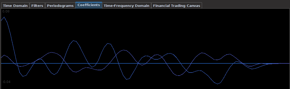
Figure : Coefficients for the TM and DIG log-return series.

Figure 12: Coefficients for the TM and DIG log-return series.

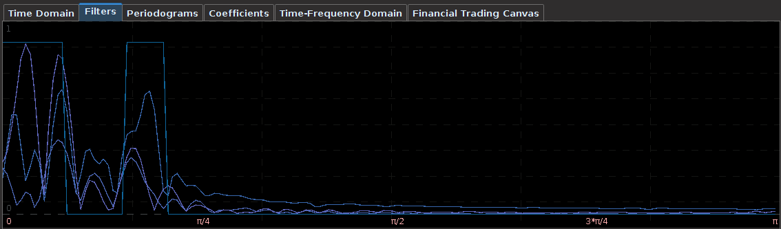
Figure : The transfer functions for the TM and DIG filter coefficients.

Figure 13: The transfer functions for the TM and DIG filter coefficients.

The coefficients for the TM and DIG series depicted in Figure 12 show the heavy amount of smooth and decay (and decay2) regularization, a trio of parameters that was not easy to pinpoint at first without significant leakage above one in the filter transfer functions (shown in Figure 13). One can see that two major spectral peaks are present under the lowpass portion and another large one in the bandpass portion that accounts for the more frequent trades.

Conclusion

With these trading signals constructed for these five assets, I imagine I have a small but somewhat diverse portfolio, ranging from tech and auto to two popular commodities. I’ll be tracking the performance of these trading signals together combined as a portfolio over the next few months and continuously give updates. As the in-sample periods for the construction of these filters ended around the end of last summer and were already applied to out-of-sample periods ranging from 90 days to 124 (roughly one half to one third of the original in-sample period), with the significant amount of regularization applied, I am quite optimistic that the out-of-sample performance will continue to be the same over the next few months, but of course one can never be too sure of anything when it comes to market behavior. In the worse case scenario, I can always look into digging though my dynamic adaptive filtering and signal extraction toolkit.

Some general comments as I conclude this article. What I truly enjoy about these trading signals constructed for this portfolio experiment (and robust trading signals in general per my other articles on financial trading) is that when any losses out-of-sample or even in-sample occur, they tend to be extremely small relative to the average size of the gains. That is the sign of a truly robust signal I suppose; that not only does it perform consistently both in-sample and out-of-sample, but also that when losses do arrive, they are quite small. One characteristic that I noticed in all robust and high performing trading signals that I tend to stick with is that no matter what type of extraction definition you are targeting (lowpass, bandpass, or MBP), when an erroneous trade is executed (leading to a loss), the signal will quickly correct itself to minimize the loss. This is why the losses in robust signals tend to be small (look at any of the 5 trading signals produced for the portfolio in this article). Of course, all these good trading signal characteristics are in addition to the filter characteristics (smooth, slightly decaying coefficients with minimal effective degrees of freedom, transfer functions less than or equal to one everywhere, etc.)

Overall, although I’m quite inspired and optimistic with these results. there is still slight room for improvement in building these MBP filters, especially for low volatility sideways markets (for example, the one occurring in the Toyota stock price in the middle of the plot in Figure 11). In general, this is a difficult type of stock price movement in which any type of signal will have success. With low volatility and no trending movements, the log-returns are basically white noise – there is no pertinent information to extract. The markets are currently efficient and there is nothing you can do about it. Only good luck will win (in that case you’re as well off building a signal based on a coin flip). Typically the best you can do in these types of areas is prevent trading altogether with some sort of threshold on the signal, which is an idea I’ve had in my mind recently but haven’t implemented, or make sure any losses are small, which is exactly what my signal achieved in Figure 11 (and which is what any robust signal should do in the first place.)

Lastly, if you have a particular financial asset for which you would like to build a trading signal (similar to the examples shown above), I will be happy to take a stab at it using iMetrica (and/or give you pointers in the right direction if you would prefer to pursue the endeavor yourself). Just send me what asset you would like to trade on, and I’ll build the filter and send you the coefficients along with the parameters used. Offer holds for a limited time only!

Happy extracting.

The Frequency Effect Part III: Revelations of Multi-Bandpass Filters and Signal Extraction for Financial Trading

Posted on January 11, 2013 by Christian Dallas Blakely

Animation of the out-of-sample performance of one of the multibandpass filters built in this article for the daily returns of the price of Google. The resulting trading signal was extracted and yielded a trading performance near 39 percent ROI during an 80 day out-of-sample period on trading shares of Google.

To conclude the trilogy on this recent voyage through various variations on frequency domain configurations and optimizations in financial trading using MDFA and iMetrica, I venture into the world of what I call multi-bandpass filters that I recently implemented in iMetrica. The motivation of this latest endeavor in highlighting the fundamental importance of the spectral frequency domain in financial trading applications was wanting to gain better control of extracting signals and engineering different trading strategies through many different types of market movement in financial assets. There are typically four different basic types of movement a price pattern will take during its fractalesque voyage throughout the duration that an asset is traded on a financial market. These patterns/trajectories include

steady up-trends in share price
low volatility sideways patterns (close to white noise)
highly volatile sideways patterns (usually cyclical)
long downswings/trends in share price.

Using MDFA for signal extraction in financial time series, one typically indicates an a priori trading strategy through the design of the extractor, namely the target function $\Gamma(\omega)$ (see my previous two articles on The Frequency Effect). Designating a lowpass or bandpass filter in the frequency domain will give an indication of what kind of patterns the extracted trading signal will trade on. Traditionally one can set a lowpass with the goal of extracting trends (with the proper amount of timeliness prioritized in the parameterization), or one can opt for a bandpass to extract smaller cyclical events for more systematic trading during volatile periods. But now suppose we could have the best of both worlds at the same time. Namely, be profitable in both steady climbs and long tumbles, while at the same time systematically hacking our way through rough sideways volatile territory, making trades at specific frequencies embedded in the share price actions not found in long trends. The answer is through the construction of multi-band pass filters. Their construction is relatively simple, but as I will demonstrate in this article with many examples, they are a bit more difficult to pinpoint optimally (but it can be done, and the results are beautiful… both aesthetically and financially).

With the multi-bandpass defined as two separate bands given by $A := 1_{[\omega_0, \omega_1]}$ , $B := 1_{[\omega_2, \omega_3]}$ with $0 \leq \omega_0$ and $\omega_1 < \omega_2$ , zero everywhere else, it is easy to see that the motivation here is to seek a detection of both lower frequencies and low-mid frequencies in the data concurrently. With now up to four cutoff frequencies to choose from, this adds yet another few wrinkles in the degrees of freedom in parameterizing the MDFA setup. If choosing and optimizing one cutoff frequency for a simple low-pass filter in addition to customization and regularization parameters wasn’t enough, now imagine extracting signals with the addition of up to three more cutoff frequencies. Despite these additional degrees of freedom in frequency interval selection, I will later give a couple of useful hacks that I’ve found helpful to get one started down the right path toward successful extraction.

With this multi-bandpass definition for $\Gamma$ comes the responsibility to ensure that the customization of smoothness and timeliness is adjusted for the additional passband. The smoothing function $W(\omega; \alpha)$ for $\alpha \geq 0$ that acts on the periodogram (or discrete Fourier transforms in multivariate mode) is now defined piecewise according to the different intervals $[0,\omega_0]$ , $[\omega_1, \omega_2]$ , and $[\omega_3, \pi]$ . For example, $\alpha = 20$ gives a piecewise quadratic weighting function (an example shown in Figure 1) and for $\alpha = 10$ , the weighting function is piecewise linear. In practice, the piecewise power function smooths and rids of unwanted frequencies in the stop band much better than using a piecewise constant function. With these preliminaries defined, we now move on to the first steps in building and applying multiband pass filters.

Figure 1: Plot of the Piecewise Smoothing Function for alpha = 15 on a mutli-band pass filter.

To motivate this newly customized approach to building financial trading signals, I begin with a simple example where I build a trading signal for the daily share price of Google. We begin with a simple lowpass filter defined by $\Gamma(\omega) = 1$ if $\omega \in [0,.17]$ , and 0 otherwise. This formulation, as it includes the zero frequency, should provide a local bias as well as extract very slow moving trends. The trick with these filters for building consistent trading performance is ensure a proper grip on the timeliness characteristics of the filter in a very low and narrow filter passage. Regularization and smoothness using the weighting function shouldn’t be too much of a problem or priority as typically just only a small fraction of the available degrees of freedom on the frequency domain are being utilized, so not much concern for overfitting as long as you’re not using too long of a filter. In my example, I maxed out the timeliness $\lambda$ parameter and set the $\lambda_{smooth}$ regularization parameter to .3. Fortunately, no optimization of any parameter was needed in this example, as the performance was spiffy enough nearly right after gauging the timeliness parameter $\lambda$ . Figure 2 shows the resulting extracted trend trading signal in both the in-sample portion (left of the cyan colored line) and applied to 80 out-of-sample points (right of the cyan line, the most recent 80 daily returns of Google, namely 9-29-12 through today, 1-10-13). The blue-pink line shows the progression of the trading account, in return-on-investment percentage. The out-of-sample gains on the trades made were 22 percent ROI during the 80 day period.

Figure 1: The in-sample and out-of-sample gains made by constructing a low-pass filter employing a very high timeliness parameter and small amount of regularization in smoothness. The out-of-sample gains are nearly 30 percent and no losses on any trades.

Figure 2: The in-sample and out-of-sample gains made by constructing a low-pass filter employing a very high timeliness parameter and small amount of regularization in smoothness. The out-of-sample gains are nearly 30 percent and no losses on any trades.

Although not perfect, the trading signal produces a monotonic performance both in-sample and out-of-sample, which is exactly what you strive for when building these trend signals for trading. The performance out-of-sample is also highly consistent (in regards to trading frequency and no losses on any trades) with the in-sample performance. With only 4 trades being made, they were done at very interesting points in the trajectory of the Google share price. Firstly, notice that the local bias in the largest upswing is accounted for due to the inclusion of frequency zero in the low pass filter. This (positive) local bias continues out-of-sample until, interestingly enough, two days before one of the largest losses in the share price of Google over the past couple years. A slightly earlier exit out of this long position (optimally at the peak before the down turn a few days before) would have been more strategic; perhaps further tweaking of various parameters would have achieved this, but I happy with it for now. The long position resumes a few days after the dust settles from the major loss, and the local bias in the signal helps once again (after trade 2). The next few weeks sees shorter downtrending cyclical effects, and the signal fortunately turns positively increasingly right before another major turning point for an upswing in the share price. Finally, the third transaction ends the long position at another peak (3), perfect timing. The fourth transaction (no loss or gain) was quickly activated after the signal saw another upturn, and thus is now in the long position (hint: Google trending upward). 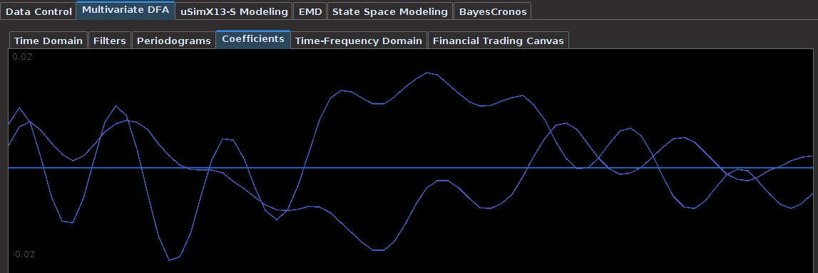Figure 3 shows the transfer functions $\hat{\Gamma}$ for both the sets of explanatory log-return data and Figure 4 depicts the coefficients for the filter. Notice that in the coefficients plot, much more weight is being assigned to past values of the log-return data with extreme (min and max values) at around lags 15 and 30 for the GOOG coefficients (blue-ish line). The coefficients are also quite smooth due to the slight amount of smooth regularization imposed.

Figure 3: Transfer functions for the concurrent trend filter applied to GOOG.

Figure 4: The filter coefficients for the log-return data.

Now suppose we wish to extract a trading signal that performs like a trend signal during long sweeping upswings or downswings, and at the same time shares the property that it extracts smaller cyclical swings during a sideways or highly volatile period. This type of signal would be endowed with the advantage that we could engage in a long position during upswings, trade systematically during sideways and volatile times, and on the same token avoid aggressive long-winded downturns in the price. Financial trading can’t get more optimistic then that, right? Here is where the magic of the multi-bandpass comes in. I give my general “how-to” guidelines in the following paragraphs as a step-by-step approach. As a forewarning, these signals are not easy to build, but with some clever optimization and patience they can be done.

In this new formulation, I envision not only being able to extract a local bias embedded in the log-return data but also gain information on other important frequencies to trade on while in sideways markets. To do this, I set up the lowpass filter as I did earlier on $[0,\omega_0]$ . The choice of $\omega_0$ is highly dependent on the data and should be located through a priori investigations (as I did above, without the additional bandpass).

Animation 2: Example of constructing a multiband pass using the Target Filter control panel in iMetrica. Initially, a low-pass filter is set, then the additional bandpass is added by clicking "Multi-Pass" checkbox. The location is then moved to the desired location using the scrollbars. The new filters are computed automaticall if "Auto" is checked on (lower left corner).

Click on the Animation 2: Example of constructing a multiband pass using the Target Filter control panel in iMetrica. Initially, a low-pass filter is set, then the additional bandpass is added by clicking “Multi-Pass” checkbox. The location is then moved to the desired location using the scrollbars. The new filters are computed automaticall if “Auto” is checked on (lower left corner).

Before setting any parameterization regarding customization, regularization, or filter constraints, I perform a quick scan of the periodogram (averaged periodogram if in multivariate mode) to locate what I call principal trading frequencies in the data. In the averaged periodogram, these frequencies are located at the largest spectral peaks, with the most useful ones for our purposes of financial trading typically before $\pi/4$ . The largest of these peaks will be defined from here on out as the principal spectral peak (PSP). Figure 6 shows an example of an averaged periodogram of the log-return for GOOG and AAPL with the PSP indicated. You might note that there exists a much larger spectral peak located at $7\pi/12$ , but no need to worry about that one (unless you really enjoy transaction costs). I locate this PSP as a starting point for where I want my signal to trade.

Figure 5: Principal spectral peak in the log-return data of GOOG and AAPL.

In the next step, I place a bandpass of width around .15 so that the PSP is dead-centered in the bandpass. Fortunately with iMetrica, this is a seamlessly simple task with just the use of a scrollbar to slide the positioning of this bandpass (and also adjust the lowpass) to where I desire. Animation 2 above (click on it to see the animation) shows this process of setting a multi-passband in the MDFA Target Filter control panel. Notice as I move the controls for the location of the bandpass, the filter is automatically recomputed and I can see the changes in the frequency response functions $\hat{\Gamma}$ instantaneously.

With the bandpass set along with the lowpass, we can now view how the in-sample performance is behaving at the initial configuration. Slightly tweaking the location of the bandpass might be necessary (width not so much, in my experience between .15 and .20 is sufficient). The next step in this approach is now to not only adjust for the location of the bandpass while keeping the PSP located somewhat centered, but also adding the effects of regularization to the filter as well. With this additional bandpass, the filter has a tendency to succumb to overfitting if one is not careful enough.

In my first filter construction attempt, I placed my bandpass at $[.49,.65]$ with the PSP directly under it. I then optimized the regularization controls in-sample (a feature I haven’t discussed yet) and slightly tweaked the timeliness parameter (ended up setting it to 3) and my result (drumroll…) is shown in Figure 6.

Figure 6: The trading performance and signal for the initial attempt at a building a multiband pass fitler.

Not bad for a first attempt. I was actually surprised at how few trades there were out-of-sample. Although there are no losses during the 80 days out-of-sample (after cyan line), and the signal is sort of what I had in mind a priori, the trades are minimal and not yielding any trading action during the period right after the large loss in Google when the market was going sideways and highly volatile. Notice that the trend signal gained from the lowpass filter indeed did its job by providing the local bias during the large upswing and then selling directly at the peak (first magenta dotted line after the cyan line). There are small transactions (gains) directly after this point, but still not enough during the sideways market after the drop. I needed to find a way to tweak the parameters and/or cutoff to include higher frequencies in the transactions.

In my second attempt, I kept the regularization parameters as they were but this time increased the bandpass to the interval $[.51, .68]$ , with the PSP still underneath the bandpass, but now catching on to a few more higher frequencies then before. I also slightly increased the length of the filter to see if that had any affect. After optimizing on the timeliness parameter $\lambda$ in-sample, I get a much improved signal. Figure 7 shows this second attempt.

Figure 7: The trading performance and signal for the second attempt at construction a multiband pass filter. This one included a few more higher frequencies.

Upon inspection, this signal behaves more consistently with what I had in mind. Notice that directly out-of-sample during the long upswing, the signal (barely) shows signs of the local bias, but enough not to make any trades fortunately. However, in this signal, we see that filter is much too late in detecting the huge loss posted by Google, and instead sells immediately after (still a profit however). Then during the volatile sideways market, we see more of what we were wishing for; timely trades to the earn the signal a quick 9 percent in the span of a couple weeks. Then the local bias kicks in again and we see not another trade posted during this short upswing, taking advantage of the local trend. This signal earned a near 22 percent ROI during the 80 day out-of-sample trading period, however not as good as the previous signal at 32 percent ROI.

Now my priority was to find another tweak that I could perform to change the trading structure even more. I’d like it to be even more sensitive to quick downturns, but at the same time keep intact the sideways trading from the signal in Figure 7. My immediate intuition was to turn on the i2 filter constraint and optimize the time-shift, similar to what I did in my previous article, part deux of the Frequency Effect. I also lessened the amount of smoothing from my weighting function $W(\omega; \alpha)$ , turned off any amount of decay regularization that I had and voila, my final result in Figure 8.

Figure 8: Third attempt at building a multiband pass filter. Here, I turn on i2 filter constraint and optimize the time shift.

While the consistency with the in-sample performance to out-of-sample performance is somewhat less than my previous attempts, out-of-sample performs nearly exactly how I envisioned. There are only two small losses of less than 1 percent each, and the timeliness of choosing when to sell at the tip of the peak in the share price of Google couldn’t have been better. There is systematic trading governed by the added multiband pass filter during the sideways and slight upswing toward the end. Some of the trades are made later than what would be optimal (the green lines enter a long position, magenta sells and enters short position), but for the most part, they are quite consistent. It’s also very quick in pinpointing its own erronous trades (namely no huge losses in-sample or out of sample). There you have it, a near monotonic performance out-of-sample with 39 percent ROI.

In examining the coefficients of this filter in Figure 9, we see characteristics of a trend filter as coefficients are largely weighting the middle lags much more than than initial or end lags (note that no decay regularization was added to this filter, only smoothness) . While at the same time however, the coefficients also weight the most recent log-return observations unlike the trend filter from Figure 4, in order to extract signals for the more volatile areas. The undulating patterns also assist in obtaining good performance in the cyclical regions.

Figure 9: The coefficients of the final filter depicting characteristics of both a trend and bandpass filter, as expected.

Finally, the frequency response functions of the concurrent filters show the effect of including the PSP in the bandpass (figure 10). Notice, the largest peak in the bandpass function is found directly at the frequency of the PSP, ahh the PSP. I need to study this frequency with more examples to get a more clear picture to what it means. In the meantime, this is the strategy that I would propose. If you have any questions about any of this, feel free to email me. Until next time, happy extracting!

Figure 10: The frequency response functions of the multiband filter.

Figure 10: The frequency response functions of the multi-bandpass filter.

The Frequency Effect: How to Infer Optimal Frequencies in Financial Trading

Posted on December 31, 2012 by Christian Dallas Blakely

Animation 1: Click to view animation. Periodogram and Various Frequency Intervals.

Animation 2: The in-sample performance of the trading signal for each frequency sweep shown in the animation above.

Animation 2: Click to view the animation. The in-sample performance of the trading signal for each frequency sweep shown in the animation above.

When constructing signals for buy/sell trades in financial data, one of the primary parameters that should be resolved before any other parameters are regarded is the trading frequency structure that regulates all the trades. The structure should be robust and consistent during all regimes of behavior for the given traded asset, namely during times of high volatility, sideways, or bull/bear markets. In the MDFA approach to building trading signals, the trading structure is mostly determined by the characteristics of the target transfer function, the $\Gamma(\omega)$ function that designates the areas of pass and stop-band frequencies in the data. As I argue in this article, I demonstrate that there exists an optimal frequency band in which the trades should be made, and the frequency band is intrinsic to the financial data being analyzed. Two assets do not necessarily share the same optimal frequency band. Needless to say, this frequency band is highly dependent on the frequency of the observations in the data (i.e. minute, hourly, daily) and the type of financial asset. Unfortunately, blindly seeking such an optimal trading frequency structure is a daunting and challenging task in general. Fortunately, I’ve built a few useful tools in the iMetrica financial trading platform to seamlessly navigate towards carving out the best (optimal or at least near optimal) trading frequency structure for any financial trading scenario. I show how it’s done in this article.

We first briefly summarize the procedure for building signals with a targeted range of frequencies in the (multivariate) direct filter approach, and then proceed to demonstrate how it is easily achieved in iMetrica. In order to construct signals of interest in any data set, a target transfer function must first be defined. This target filter transfer function $\Gamma(\omega)$ defined on $\omega \in [0,\pi]$ controls the frequency content of the output signal through the computation of the optimal filter coefficients. Defining $\hat{\Gamma}(\omega) = \sum_{j=0}^{L-1} b_j \exp(i j \omega)$ for some collection of filter coefficients $b_j, \, j=0,\ldots,L-1$ , recall that in the plain-vanilla (univariate) direct filter approach (for ‘quasi’ stationary data), we seek to find the $L$ coefficients such that $\int_{-\pi}^{\pi} |\Gamma(\omega) - \hat{\Gamma}(\omega)|^2 H(\omega) d\omega$ is minimized, where $H(\omega)$ is a ‘smart’ weighting function that approximates the ‘true’ spectral density of the data (in general the periodogram of the data, or a function using the periodogram of the data). By defining $\Gamma(\omega)$ as a function that takes on the value of one or less for a certain range of values in $[0,\pi]$ and zero elsewhere, we pinpoint exotic frequencies where we wish our filter to extract the features of the data. The characteristics of the generated output signal (after the resulting filter has been applied to the data) are those intrinsic to the selected frequencies in the data. The characteristics found at other frequencies are (in a perfect world) disregarded from the output signal. As we show in this article, the selection of the frequencies when defining $\Gamma(\omega)$ provides the utmost in importance when building financial trading signals, as the optimal frequencies in regards to trading performance vary with every data set.

As mentioned, much emphasis should be applied to the construction of this target $\Gamma(\omega)$ and finding the optimal one is not necessarily an easy task in general. With a plethora of other parameters that are involved in building a trading signal, such as customization and regularization (see my article on financial trading parameters), one could just simply select any arbitrary frequency range for $\Gamma(\omega)$ and then proceed to optimize the other parameters until a winning trading signal is found. That is, of course, an option. But I’d like to be an advocate for carving out the proper frequency range that’s intrinsically optimal for the data set given, namely because I believe one exists, and secondly because once in the proper frequency range for the data, other parameters are much easier to optimize. So what kind of properties should this ‘optimal’ frequency range possess in regards to the trading signal?

Consistency. Provides out-of-sample performance akin to in-sample performance.
Optimality. Generates in-sample trade performance with rank coefficient above .90.
Robustness. Insensitive to small changes in parameterization.

Most of these properties are obvious when first glancing at them, but are completely nontrivial to obtain. The third property tends to be overlooked when building efficient trading signals as one typically chooses a parameterization for a specific frequency band in the target $\Gamma(\omega)$ , and then becomes over-confident and optimistic that the filter will provide consistent results out-of-sample. With a non-robust signal, small change in one of the customization parameters completely eradicates the effectiveness and optimality of the filter. An optimal frequency range should be much less sensitive to changes in the customization and regularization of the filter parameters. Namely, changing the smoothing parameter, say 50 percent in either direction, will have little effect on the in-sample performance of the filter, which in turn will produce a more robust signal.

To build a target transfer function $\Gamma(\omega)$ , one has many options in the MDFA module of iMetrica. The approach that we will consider in this article is to define $\Gamma(\omega)$ directly by indicating the frequency pass-band and stop-band structure directly. The simplest transfer functions are defined by two cutoff frequencies: a low cutoff frequency $\omega_0$ and a high-cutoff frequency $\omega_1$ . In the Target Filter Design control panel (see Figure 1), one can control every aspect of the target transfer function $\Gamma(\omega)$ function, from different types of step functions, to more exotic options using modeling. For building financial trading signals, the Band-Pass option will be sufficient. The cutoff frequencies $\omega_0$ and $\omega_1$ are adjusted by simply modifying their values using the slider bars designated for each value, where three different ways of modifying the cutoff frequency values are available. The first is the direct designation of the value using the slider bar which goes between values of $(0,\pi)$ by changes of .01. The second method uses two different slider bars to change the values of the numerator $n$ and denominator $d$ where $\omega_0$ and/or $\omega_1$ is written in fractional form $2\pi n/d$ , a form commonly used for defining different cycles in the data. The third method is to simply type in the value of the cutoff in the designated text area and then press Enter on the keyboard, where the number must be a real number in the interval $(0,\pi)$ and entered in decimal form (i.e. 0.569, 1.349, etc). When the Auto checkbox is selected, the new direct filter and signal will be computed automatically when any changes to the target transfer function are made. This can be a quite useful tool for robustness verification, to see how small changes in the frequency content affect the output signal, and consequently the trading performance of the signal.

Figure 1: Target filter design panel.

Although cycling through multiple frequency ranges to find the optimal frequency bands for in-sample trading performance can be seamlessly accomplished by just sliding the scrollbars around (as shown in Animations 1 and 2 at the top of the page), there is a much easier way to achieve optimality (or near optimality) automatically thanks to a Financial Trading Optimization control panel featured in the Financial Trading menu at the top of the iMetrica interface. Once in the Financial Trading interface, optimization of both the customization parameters for timeliness and smoothness, along with optimization of the $\Gamma(\omega)$ frequency bands can be accomplished by first launching the Trading Optimization panel (see Figure 2), and then selecting the optimization criteria desired (maximum return, minimum loss, maximum trade success ratio, maximum rank coefficient,… etc). 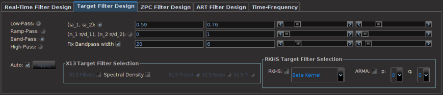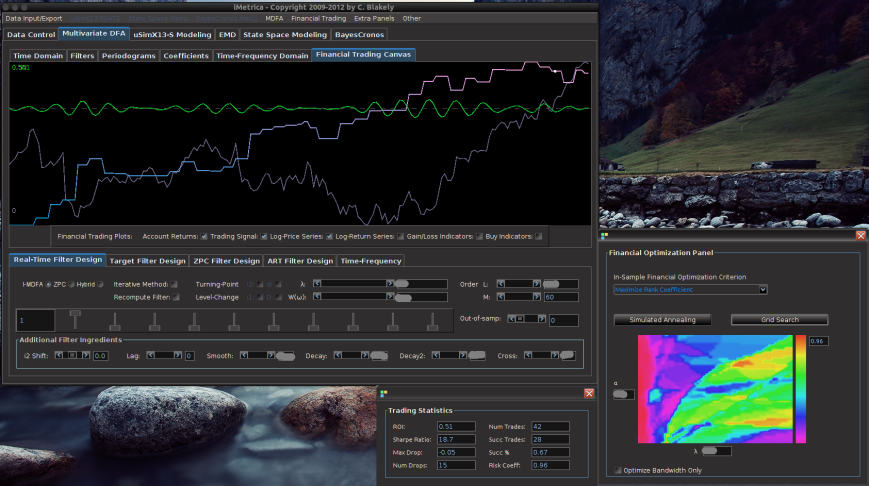To find the optimal customization parameters, simply select the optimization criteria from the drop-down menu, and then click either the Simulated Annealing button, or Grid Search button (as the name implies, ‘grid search’ simply creates a fine grid of customization values $\lambda$ and smoothing expweight $\alpha$ and then chooses the maximal value after sweeping the entire grid – it takes a few seconds depending on the length of the filter. The method that I prefer for now). After the optimal parameters are found, the plotting canvas in the optimization panel paints a contour plot of the values found in order to give you an idea of the customization geometry, with all other parameterization values fixed. The frequency bandwidth of the target transfer function can then be optimized by a quick few millisecond grid search by selecting the checkbox Optimize bandwidth only. In this case the customization parameters are held fixed to their set values, and the optimization proceeds to only vary the frequency parameters. The values of the optimization function produced during the grid-search are then plotted on the optimization canvas to yield the structure from the frequency domain point-of-view. This can be helpful when comparing different frequency bands in building trading signals. It can also help in determining the robustness of the signal, by looking at the near neighboring values found at the optimal value.

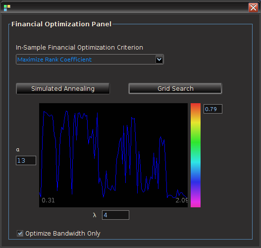
Figure 2: The financial trading optimization panel. Here the values of the optimization criteria are plotted for all the different frequency intervals. The interval with the maximum value is automatically chosen and then computed.

We give a full example of an actual trading scenario to show how this process works in selecting an optimal frequency range for a given set of market traded assets. The outline of my general step-by-step approach for seeking good trading filters goes as follows.

Select the initial frequency band-pass by first initializing the $(\omega_1, \omega_2)$ interval to $(0, \omega_2)$ . Setting $\omega_2$ to .10-.15 is usually sufficient. Set the checkbox Fix-Bandpass width in order to secure the bandwidth of the filter.
In the optimization panel (Figure 2), click the checkbox Optimize Bandwidth only and then select the optimization criteria. In these examples, we choose to maximize the rank coefficient, as it tends to produce the best out-of-sample trading performance. Then tap the Grid Search button to find the frequency range with the maximum rank coefficient. This search takes a few milliseconds.
With the initialization of the optimal bandwidth, the customization parameters can now be optimized by deselecting the Optimize Bandwidth only and then tapping the Grid Search button once more. Depending on the length of the filter $L$ and the number of addition explaining series, this search can take several seconds.
Repeat steps 2 and 3 until a combination is found of customization and filter bandwidth that produces a rank coefficient above .90. Also, test the robustness of the trading signal by slightly adjusting the frequency range and the customization parameters by small changes. A robust signal shouldn’t change the trading statistics too much under slight parameter movement.

Once content with the in-sample trading statistics (the Trading Statistics panel is available from the Financial Trading Menu), the final step is to apply the filter to out-of-sample data and trade away. Provided that sufficient regularization parameters have been selected prior to the optimization (regularization selection is out of the scope of this article however) and the optimized trading frequency bandwidth was robust enough, the out-of-sample performance of the signal should perform akin to in-sample. If not, start over with different regularization parameters and filter length, or seek options using adaptive filtering (see my previous article on adaptive filtering).

In our example, we trade on the daily price of GOOG by using GOOG log-return data as the target data and first explanatory series, along with AAPL daily log-returns as the second explanatory series. After the four steps taken above, an optimal frequency range was found to be $(.63,.80)$ , where the in-sample period was from 6-3-2011 to 9-21-2012. The post-optimization of the filter, showing the MDFA trading interface, the in-sample trading statistics, and the trading optimization is shown in Figure 3. Here, the in-sample maximum rank coefficient was found to be at .96 (1.0 is the best, -1.0 is pitiful), where the trade success ratio is around 67 percent, a return-on-investment at 51 percent, and a maximum loss during the in-sample period at around 5 percent. Applying this filter out-of-sample on incoming data for 30 trading days, without any adjustments to the filter, we see that the performance of the signal was very much akin to the performance in-sample (see Figure 5). At the end of the 30 out-of-sample trading days after the in-sample period, the trading signal gives a 65 percent return for a total of a 14 percent return-on-investment in 30 trading days. During this period, there were 6 trades made (3 buys and 3 sell shorts), and 5 of them were successful (with a .1 percent transaction cost for any trade), which amounts to, on average, one trade per week.

Figure 3. After in-sample optimization on both the customization and filter frequency band.

Figure 4: After applying the constructed filter on the next 30 days out-of-sample.

The other filter parameters (customization, regularization, and filter length $L$ ) have been blurred-out on purpose for obvious reasons. However, interested readers can e-mail me and I’ll send the optimal customization and regularization parameters, or maybe even just the filter coefficients themselves so you can apply them to data future GOOG and AAPL data and experiment.) We then apply the filter out-of-sample for 30 days and make trades based on the output of the trading signal. In Figure 4, the blue-to-pink line represents the performance of the trading account given by the percentage returns from each trade made over time. The grey line is the log-price of GOOG, and the green line is the trading signal constructed from the filter just built applied to the data. It signals a ‘buy’ when the signal moves above the zero line (the dotted line) and a sell (and short-sell) when below the line. Since the data are the daily log-returns at the end each market trading period, all trades are assumed to have been made near or at the end of market hours.

Notice how successful this chosen frequency range is during the times of highest volatility for Google being in this example the first 60 day period of the in-sample partition (roughly September-October 2011). This in-sample optimization ultimately helped the 30 days out-of-sample period where volatility increased again (with even an 8 percent drop on October 17th, 2012). Out of all the largest drops in the price of Google in both the in-sample and out-of-sample period, the signal was able to anticipate all of them due to the smart choice of the frequency band and then end up making profits by short-selling.

To summarize, during an out-of-sample period in which GOOG lost over 10 percent of their stock price, the optimized trading signal that was built in this example earned roughly 14 percent. We were able to accomplish this by investigating the properties of the behavior of different frequency intervals in regard to not only the optimization criteria, but also areas of robustness in both the values of the filter frequency intervals as well as customization controls (see the animations at the top of this article). This is mostly aided by the very efficient and fast (this is where the gnu-c language came in handy) financial trading optimization panel as well as the ability in iMetrica to make any changes to the filter parameters and instantaneously see the results. Again, feel free to contact me for the filter parameters that were found in the above example, the filter coefficients, or any questions you may have.

Happy New Year and Happy Extracting!

Hybrid Signal Extraction, Machine Learning, and Algorithmic Financial Trading

Combining Computational Methodologies for Real-Time Learning and Signal Extraction

Tag Archives: Fourier Analysis