The Frequency Effect: How to Infer Optimal Frequencies in Financial Trading

Posted on December 31, 2012 by Christian Dallas Blakely

Animation 1: Click to view animation. Periodogram and Various Frequency Intervals.

Animation 2: The in-sample performance of the trading signal for each frequency sweep shown in the animation above.

Animation 2: Click to view the animation. The in-sample performance of the trading signal for each frequency sweep shown in the animation above.

When constructing signals for buy/sell trades in financial data, one of the primary parameters that should be resolved before any other parameters are regarded is the trading frequency structure that regulates all the trades. The structure should be robust and consistent during all regimes of behavior for the given traded asset, namely during times of high volatility, sideways, or bull/bear markets. In the MDFA approach to building trading signals, the trading structure is mostly determined by the characteristics of the target transfer function, the $\Gamma(\omega)$ function that designates the areas of pass and stop-band frequencies in the data. As I argue in this article, I demonstrate that there exists an optimal frequency band in which the trades should be made, and the frequency band is intrinsic to the financial data being analyzed. Two assets do not necessarily share the same optimal frequency band. Needless to say, this frequency band is highly dependent on the frequency of the observations in the data (i.e. minute, hourly, daily) and the type of financial asset. Unfortunately, blindly seeking such an optimal trading frequency structure is a daunting and challenging task in general. Fortunately, I’ve built a few useful tools in the iMetrica financial trading platform to seamlessly navigate towards carving out the best (optimal or at least near optimal) trading frequency structure for any financial trading scenario. I show how it’s done in this article.

We first briefly summarize the procedure for building signals with a targeted range of frequencies in the (multivariate) direct filter approach, and then proceed to demonstrate how it is easily achieved in iMetrica. In order to construct signals of interest in any data set, a target transfer function must first be defined. This target filter transfer function $\Gamma(\omega)$ defined on $\omega \in [0,\pi]$ controls the frequency content of the output signal through the computation of the optimal filter coefficients. 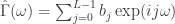Defining $\hat{\Gamma}(\omega) = \sum_{j=0}^{L-1} b_j \exp(i j \omega)$ for some collection of filter coefficients $b_j, \, j=0,\ldots,L-1$ , recall that in the plain-vanilla (univariate) direct filter approach (for ‘quasi’ stationary data), we seek to find the $L$ coefficients such that $\int_{-\pi}^{\pi} |\Gamma(\omega) - \hat{\Gamma}(\omega)|^2 H(\omega) d\omega$ is minimized, where $H(\omega)$ is a ‘smart’ weighting function that approximates the ‘true’ spectral density of the data (in general the periodogram of the data, or a function using the periodogram of the data). By defining $\Gamma(\omega)$ as a function that takes on the value of one or less for a certain range of values in $[0,\pi]$ and zero elsewhere, we pinpoint exotic frequencies where we wish our filter to extract the features of the data. The characteristics of the generated output signal (after the resulting filter has been applied to the data) are those intrinsic to the selected frequencies in the data. The characteristics found at other frequencies are (in a perfect world) disregarded from the output signal. As we show in this article, the selection of the frequencies when defining $\Gamma(\omega)$ provides the utmost in importance when building financial trading signals, as the optimal frequencies in regards to trading performance vary with every data set.

As mentioned, much emphasis should be applied to the construction of this target $\Gamma(\omega)$ and finding the optimal one is not necessarily an easy task in general. With a plethora of other parameters that are involved in building a trading signal, such as customization and regularization (see my article on financial trading parameters), one could just simply select any arbitrary frequency range for $\Gamma(\omega)$ and then proceed to optimize the other parameters until a winning trading signal is found. That is, of course, an option. But I’d like to be an advocate for carving out the proper frequency range that’s intrinsically optimal for the data set given, namely because I believe one exists, and secondly because once in the proper frequency range for the data, other parameters are much easier to optimize. So what kind of properties should this ‘optimal’ frequency range possess in regards to the trading signal?

Consistency. Provides out-of-sample performance akin to in-sample performance.
Optimality. Generates in-sample trade performance with rank coefficient above .90.
Robustness. Insensitive to small changes in parameterization.

Most of these properties are obvious when first glancing at them, but are completely nontrivial to obtain. The third property tends to be overlooked when building efficient trading signals as one typically chooses a parameterization for a specific frequency band in the target $\Gamma(\omega)$ , and then becomes over-confident and optimistic that the filter will provide consistent results out-of-sample. With a non-robust signal, small change in one of the customization parameters completely eradicates the effectiveness and optimality of the filter. An optimal frequency range should be much less sensitive to changes in the customization and regularization of the filter parameters. Namely, changing the smoothing parameter, say 50 percent in either direction, will have little effect on the in-sample performance of the filter, which in turn will produce a more robust signal.

To build a target transfer function $\Gamma(\omega)$ , one has many options in the MDFA module of iMetrica. The approach that we will consider in this article is to define $\Gamma(\omega)$ directly by indicating the frequency pass-band and stop-band structure directly. The simplest transfer functions are defined by two cutoff frequencies: a low cutoff frequency $\omega_0$ and a high-cutoff frequency $\omega_1$ . In the Target Filter Design control panel (see Figure 1), one can control every aspect of the target transfer function $\Gamma(\omega)$ function, from different types of step functions, to more exotic options using modeling. For building financial trading signals, the Band-Pass option will be sufficient. The cutoff frequencies $\omega_0$ and $\omega_1$ are adjusted by simply modifying their values using the slider bars designated for each value, where three different ways of modifying the cutoff frequency values are available. The first is the direct designation of the value using the slider bar which goes between values of $(0,\pi)$ by changes of .01. The second method uses two different slider bars to change the values of the numerator $n$ and denominator $d$ where $\omega_0$ and/or $\omega_1$ is written in fractional form $2\pi n/d$ , a form commonly used for defining different cycles in the data. The third method is to simply type in the value of the cutoff in the designated text area and then press Enter on the keyboard, where the number must be a real number in the interval $(0,\pi)$ and entered in decimal form (i.e. 0.569, 1.349, etc). When the Auto checkbox is selected, the new direct filter and signal will be computed automatically when any changes to the target transfer function are made. This can be a quite useful tool for robustness verification, to see how small changes in the frequency content affect the output signal, and consequently the trading performance of the signal.

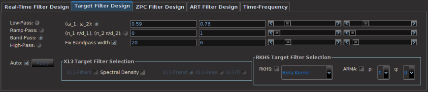
Figure 1: Target filter design panel.

Although cycling through multiple frequency ranges to find the optimal frequency bands for in-sample trading performance can be seamlessly accomplished by just sliding the scrollbars around (as shown in Animations 1 and 2 at the top of the page), there is a much easier way to achieve optimality (or near optimality) automatically thanks to a Financial Trading Optimization control panel featured in the Financial Trading menu at the top of the iMetrica interface. Once in the Financial Trading interface, optimization of both the customization parameters for timeliness and smoothness, along with optimization of the $\Gamma(\omega)$ frequency bands can be accomplished by first launching the Trading Optimization panel (see Figure 2), and then selecting the optimization criteria desired (maximum return, minimum loss, maximum trade success ratio, maximum rank coefficient,… etc). To find the optimal customization parameters, simply select the optimization criteria from the drop-down menu, and then click either the Simulated Annealing button, or Grid Search button (as the name implies, ‘grid search’ simply creates a fine grid of customization values $\lambda$ and smoothing expweight $\alpha$ and then chooses the maximal value after sweeping the entire grid – it takes a few seconds depending on the length of the filter. The method that I prefer for now). After the optimal parameters are found, the plotting canvas in the optimization panel paints a contour plot of the values found in order to give you an idea of the customization geometry, with all other parameterization values fixed. The frequency bandwidth of the target transfer function can then be optimized by a quick few millisecond grid search by selecting the checkbox Optimize bandwidth only. In this case the customization parameters are held fixed to their set values, and the optimization proceeds to only vary the frequency parameters. The values of the optimization function produced during the grid-search are then plotted on the optimization canvas to yield the structure from the frequency domain point-of-view. This can be helpful when comparing different frequency bands in building trading signals. It can also help in determining the robustness of the signal, by looking at the near neighboring values found at the optimal value.

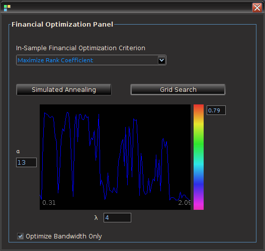
Figure 2: The financial trading optimization panel. Here the values of the optimization criteria are plotted for all the different frequency intervals. The interval with the maximum value is automatically chosen and then computed.

We give a full example of an actual trading scenario to show how this process works in selecting an optimal frequency range for a given set of market traded assets. The outline of my general step-by-step approach for seeking good trading filters goes as follows.

Select the initial frequency band-pass by first initializing the $(\omega_1, \omega_2)$ interval to $(0, \omega_2)$ . Setting $\omega_2$ to .10-.15 is usually sufficient. Set the checkbox Fix-Bandpass width in order to secure the bandwidth of the filter.
In the optimization panel (Figure 2), click the checkbox Optimize Bandwidth only and then select the optimization criteria. In these examples, we choose to maximize the rank coefficient, as it tends to produce the best out-of-sample trading performance. Then tap the Grid Search button to find the frequency range with the maximum rank coefficient. This search takes a few milliseconds.
With the initialization of the optimal bandwidth, the customization parameters can now be optimized by deselecting the Optimize Bandwidth only and then tapping the Grid Search button once more. Depending on the length of the filter $L$ and the number of addition explaining series, this search can take several seconds.
Repeat steps 2 and 3 until a combination is found of customization and filter bandwidth that produces a rank coefficient above .90. Also, test the robustness of the trading signal by slightly adjusting the frequency range and the customization parameters by small changes. A robust signal shouldn’t change the trading statistics too much under slight parameter movement.

Once content with the in-sample trading statistics (the Trading Statistics panel is available from the Financial Trading Menu), the final step is to apply the filter to out-of-sample data and trade away. Provided that sufficient regularization parameters have been selected prior to the optimization (regularization selection is out of the scope of this article however) and the optimized trading frequency bandwidth was robust enough, the out-of-sample performance of the signal should perform akin to in-sample. If not, start over with different regularization parameters and filter length, or seek options using adaptive filtering (see my previous article on adaptive filtering).

In our example, we trade on the daily price of GOOG by using GOOG log-return data as the target data and first explanatory series, along with AAPL daily log-returns as the second explanatory series. After the four steps taken above, an optimal frequency range was found to be $(.63,.80)$ , where the in-sample period was from 6-3-2011 to 9-21-2012. The post-optimization of the filter, showing the MDFA trading interface, the in-sample trading statistics, and the trading optimization is shown in Figure 3. Here, the in-sample maximum rank coefficient was found to be at .96 (1.0 is the best, -1.0 is pitiful), where the trade success ratio is around 67 percent, a return-on-investment at 51 percent, and a maximum loss during the in-sample period at around 5 percent. Applying this filter out-of-sample on incoming data for 30 trading days, without any adjustments to the filter, we see that the performance of the signal was very much akin to the performance in-sample (see Figure 5). At the end of the 30 out-of-sample trading days after the in-sample period, the trading signal gives a 65 percent return for a total of a 14 percent return-on-investment in 30 trading days. During this period, there were 6 trades made (3 buys and 3 sell shorts), and 5 of them were successful (with a .1 percent transaction cost for any trade), which amounts to, on average, one trade per week.

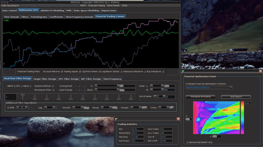
Figure 3. After in-sample optimization on both the customization and filter frequency band.

Figure 4: After applying the constructed filter on the next 30 days out-of-sample.

The other filter parameters (customization, regularization, and filter length $L$ ) have been blurred-out on purpose for obvious reasons. However, interested readers can e-mail me and I’ll send the optimal customization and regularization parameters, or maybe even just the filter coefficients themselves so you can apply them to data future GOOG and AAPL data and experiment.) We then apply the filter out-of-sample for 30 days and make trades based on the output of the trading signal. In Figure 4, the blue-to-pink line represents the performance of the trading account given by the percentage returns from each trade made over time. The grey line is the log-price of GOOG, and the green line is the trading signal constructed from the filter just built applied to the data. It signals a ‘buy’ when the signal moves above the zero line (the dotted line) and a sell (and short-sell) when below the line. Since the data are the daily log-returns at the end each market trading period, all trades are assumed to have been made near or at the end of market hours.

Notice how successful this chosen frequency range is during the times of highest volatility for Google being in this example the first 60 day period of the in-sample partition (roughly September-October 2011). This in-sample optimization ultimately helped the 30 days out-of-sample period where volatility increased again (with even an 8 percent drop on October 17th, 2012). Out of all the largest drops in the price of Google in both the in-sample and out-of-sample period, the signal was able to anticipate all of them due to the smart choice of the frequency band and then end up making profits by short-selling.

To summarize, during an out-of-sample period in which GOOG lost over 10 percent of their stock price, the optimized trading signal that was built in this example earned roughly 14 percent. We were able to accomplish this by investigating the properties of the behavior of different frequency intervals in regard to not only the optimization criteria, but also areas of robustness in both the values of the filter frequency intervals as well as customization controls (see the animations at the top of this article). This is mostly aided by the very efficient and fast (this is where the gnu-c language came in handy) financial trading optimization panel as well as the ability in iMetrica to make any changes to the filter parameters and instantaneously see the results. Again, feel free to contact me for the filter parameters that were found in the above example, the filter coefficients, or any questions you may have.

Happy New Year and Happy Extracting!

Dream within a dream: How science fiction concepts from the movie Inception can be accomplished in real life (via MDFA)

Posted on December 21, 2012 by Christian Dallas Blakely

“Careful, we may be in a model…within a model.” (From an Inception movie poster.)

Have you ever seen the movie Inception and wondered, “Gee, wouldn’t it be neat if I could do all that fancy subconscious dream within a dream manipulation stuff”? Well now you can (in a metaphorical way) using MDFA and iMetrica. I explain how in this article.

Before I begin, may I first draw your attention to a brief introduction of the context in which I am speaking, and that is real-time signal extraction in (nonlinear, nonstationary) information flow. The principle goal of filtering and signal extraction in real-time data analysis for whatever purpose necessary (financial trading, risk analysis, real-time trend detection, seasonal adjustment) is to detect and pinpoint as timely as possible a desired sequence of events in an incoming flow of data observations. We emphasize that this detection should be fast, in that the desired signal, or sequence of events, should be so robust in its timeliness and accuracy so as to detect turning points or actions in targeted events as they happen, or even become so awesome that it manages to anticipate what will happen in the future. Of course, this is never an exact science nor even always possible (otherwise we’d all be billionaires right?) and thus we rely on creative ways to cope with the unknown.

We can also think of signal extraction in more abstract terms. Real-time signal extraction entails the construction of a ‘smart’ illusion, an alternative to reality, where reality in this context is a time series, the information flow, the raw data. This ‘smart’ illusion that is being constructed is the signal, the vital information that has been extracted from an abundance of “noise” embedded in the reality. And the signal must produce important underlying secrets to satisfy the needs of the user, the signal extractor. How these signals are extracted from reality is the grand challenge. How are they produced in a robust, fast, and feasible manner so as to be effective in the real-time flow of information? The answer is in MDFA, or in other words as I’ll describe in this article, penetrating the subconscious state of reality to gain access to hidden treasures.

After recently re-watching the Christopher Nolan opus entitled Inception starring Leonardo DiCaprio and what seems like most of the cast from the Dark Knight Trilogy, I began to see some similarities between the main concepts entertainingly presented in the movie (using some pimped-up CGI), and the mathematics of signal extraction using the multivariate direct filtering approach (MDFA). In this article I present some of these interesting parallels that I’ve managed to weave together. My ultimate goal with this article is to hopefully paint a vivid picture of some interesting details stemming from the mathematics of the direct filtering approach by using the parallels that I’ve contrived between the two. Afterwards, hopefully you’ll be on your way to entering the realm of ‘dreaming within dreaming’, and extracting pertinent hidden secrets embedded in a flurry of noise.

The film introduces a slick con man by the name of Cobb (played by DiCaprio), and his team of super well-dressed con artists with leather jackets and slicked back hair (the classic con man look right?). The catchy idea that resides in the premise of the film is that these aren’t ordinary con men: they have a unique way of manipulating reality: by entering the dreams (subconscious ) of their targets (or marks as they call them in the film) and manipulate their subconscious dream state under the goal of extracting a desired idea or hidden secret. Like any group of con men, they attempt to construct a false reality by creating a certain architecture and environment in the target’s dream. The effectiveness of this ‘heist’ to capture the desired signals in the dream relies on the quality of the architecture and environment of the dream.

So how does all this relate to the mathematics of the MDFA for signal extraction. My vision can be seen as follows. In manipulating the target’s subconscious , Cobb’s group basically involves a collection of four components. Each one can be associated with a mathematical concept embedded in the MDFA.

The Target – At the highest level, we have reality. The real world in which the characters, and the target (victim), live. The target victim has an abundance of hidden information among the large capacity of mostly noise, from which Cobb’s group wish to manipulate and extract a hidden secret, the signal. In the MDFA world, we can associate or represent the information flow, the time series on which we perform the signal extraction process as the target victim in the real world. This is the data that we see, the reality. This data of course is non-deterministic, namely we have no idea what the target victim has in mind for the future. The process of extracting the hidden thoughts or ideas from this target victim is akin to, in the MDFA world, the signal extraction process. The tools used to do the extracting are as follows.

The Extractor – The extractor is depicted in Inception as a master con man, a person who knows how to manipulate a subject (the target) in their subconscious dreaming world into revealing their deepest mental secrets. As the extractor’s goal is manipulation of the subconscious of a target to reveal a certain signal buried within reality, the extractor must transform the real-world conscious mental state of the target from reality into the dreaming subconscious world, by inducing a dream state. The multivariate direct filtering process of transforming the data (reality) into spectral frequency space (the subconscious ) via the Fourier transform to reveal the signal given the desired target data is metaphorically very similar to this process. The Inception extractor can be seen as being parallel to the process of transforming the data from reality into a subconscious world, the spectral frequency domain. It’s in this dreaming subconscious world, the frequency domain, where the real manipulation begins, using an architect.

The Architect – The Inception architect is the designer of the dream who constructs and builds the subconscious world into which the extractor brings the subject, or target. Just as the architect manipulates real world architecture and physics in order to create paradoxes like an endless staircase, folding buildings, smooth transitions from one place to another and other various phenomena otherwise impossible in the real world, the architect in the filtering world is the toolkit of filtering parameters that render the finite-dimensional metric space in which one constructs the filter coefficients to produce the desired signal. This includes the extraction rules (namely the symmetric target filter), customization for timeliness and speed, and regularization to warp and bend the finite dimensional filter metric space. Just as many different paths in the subconscious world toward the manipulation of the target subject exist and it is the architect’s job to create the optimal environment for extracting the desired signal, the architect in the direct filtering world uses the wide ranging set of filter parameters to bend and manipulate the metric space from which the filter coefficients are built and then used in the signal extraction process. Just as changing dynamics in the Inception real world (like the state of free-falling) will change the physics of the dreamt subconscious world (like floating in hotel elevator shafts while engaging in physical combat, Matrix style), changing dynamics in the information flow will alter the geometry of the consequent architecture being built for the filter. And furthermore, just as the dream architect must be highly skilled in order to manipulate correctly, the MDFA architect must be highly skilled in order to construct the appropriate space in which the optimal signal is extracted (hint hint, call me or Marc, we’re the extractors and architects).

Dream within a dream – As one of the more fascinating concepts introduced in Inception, the concept of the dream within a dream was also the main trick to their success in dream manipulation. Starting from reality, each level of the dreaming subconscious state can be further transposed into another level of subconscious , namely dreaming within a dream. The dream within a dream process puts you into a deeper state of dreaming. The deeper you go, the further one’s mind is removed from reality. This is where the subject of dynamic adaptive filtering comes into play (see my previous article here for an intro and basics to dynamic adaptive filtering in iMetrica). In the direct filtering world, dynamic adaptive filtering is akin to the dream within a dream concept: Once in a level of subconscious (the spectral frequency space in MDFA), and the architect has created the dream used for manipulation (the metric space for the filter coefficients), a new level of subconscious can then be entered by introducing a newly adapted metric space based on the information extracted from the first level of subconscious.

In the dream within a dream, time is the other factor. The deeper you go into a dream state, the faster your mind is able to imagine and perceive things within that dream state. For example, one minute in reality can seem like one hour in the dream state. At the next level of subconscious, at each level in the subconscious , the element of time speeds up exponentially. A similar analogy can be extracted (no pun intended) in the concept of dynamic adaptive filtering. In dynamic adaptive filtering, we first begin by extracting a signal with the desired filter architecture at the first level transformation from reality to the spectral frequency space. When new information is received and our extracted signal is not behaving how we desire, we can build a new filter architecture for manipulating the signal with the newly provided information, with all the filter parameters available to control the desired filter properties. We are inherently building a new updated filter architecture on top of the old filter architecture, and consequently building a new signal from the output of the old signal by correcting (manipulating) this old signal toward our desired goals. This is akin to the dream within a dream concept. And just like the idea of time passing much faster at each subconscious level, the effects of filter parameters for controlling regularization and speed occur at a much faster rate since we are dealing with less information, a much shorter time frame (namely the newly arrived information) at each subsequent filtering level. One can even continue down the levels of subconscious, building a new architecture on top of the previous architecture, continuously using the newly provided information at each level to build the next level of subconsciousness; dream within a dream within a dream.

To summarize these analogies, I’ll be adding a graphic soon to this article that explains in a more succinct manner these parallels described above between Inception and MDFA. In the meantime, here are the temporary replacements.

Haters gonna hate… extractors gonna extract.

Nolan, why you leavin’ Leo out?

Dynamic Adaptive Filtering and Signal Extraction

Posted on December 20, 2012 by Christian Dallas Blakely

This slideshow requires JavaScript.

Introduction

Dynamic adaptive filtering is the method of updating a signal extraction process in real-time using newly provided information. This newly provided information is the next sequence of observed data, such as minute, hourly, or daily log-returns in a portfolio of financial assets, or a new set of weekly/monthly observations in a set of economic indicators. The goal is to improve the properties of the extracted signal with respect to a target (symmetric) filter and the output of past (old) signal values that are not performing as they should be (perhaps due to overfitting). In the multivariate direct filtering approach framework, it is an easily workable task to update the signal while only using the most recent information given. As a recently proposed idea by Marc Wildi last month, in this dynamic form of adaptive filtering we seek to update and improve a signal for a given multivariate time series information flow by computing a new set of filter coefficients to only a small window of the time series that features the latest observations. Instead of recomputing an entire new set of filter coefficients in-sample on the entire data set, we use a much smaller data set, say the latest $\tilde{N}$ observations on which the older filter was applied out-of-sample which is much less than the total number of observations in the time series.

The new filter coefficients computed on this small window of new observations uses as input the filtered series from original ‘old’ filter. These new updated coefficients are then applied to the output of the old filter, leading to completely re-optimized filter coefficients and thus an optimized signal, eliminating any nasty effects due overfitting or signal ‘overshooting’ in the older filter, while at the same time utilizing new information. This approach is akin to, in a way, filtering within filtering: the idea of ‘smart’-filtering on previously filtered data for optimized control of the new signal being computed. It could also be thought of as filtering filtered data, a convolution of filters, updating the real-time signal, or, more generally, adaptive filtering. However you wish to think of it, the idea is that a new filter provides the necessary updating by correcting the signal output of the old filter, applied to data out-of-sample. A rather smart idea as we will see. With the coefficients of the old filter are kept fixed, we enter into the frequency world of the output of the ‘old’ filter to gain information on optimizing the new filter. Only the coefficients of the new updated filter are optimized, and can be optimized anytime new data becomes available. This adaptive process is dynamic in the sense that we require new information to stream in in order to update the new signal by constructing a new filter. Once the new filter is constructed, the newly adapted signal is built by first applying the old filter to the data to produce the initial (non-updated) signal from the new data, then the newly constructed filter optimized from this output is then applied to the ‘old’ signal producing the smarter updated signal. Below is an outline of this algorithm for dynamic adaptive filtering stripped of much of the mathematical details. A more in-depth look at the mathematical details of MDFA and this newly proposed adaptive filtering method can be found in section 10.1 of the Elements paper by Wildi.

Basic Algorithm

We begin with a target time series $Y_t$ , $t=1,\ldots, N$ from which we wish to extract a signal, and along with it a set of $M$ explanatory time series $Y_{j,t}$ , $t=1,\ldots,N$ , $j=1,\ldots,M$ that may help in describing the dynamics of our target time series $Y_t$ . Note that in many applications, such as financial trading, we normally set $Y_{1,t} = Y_t$ so that our target time series is included in the explanatory time series set, which makes sense since it is the only known time series to perfectly describe itself (however, not in every signal extraction applications is this a good idea. See for example the GDP filtering work of Wildi here)To extract the initial signal in the given data set (in-sample), we define a target filter $\Gamma(\omega)$ , that lives on the frequency domain $\omega \in [0,\pi]$ . We define the architecture of the filter metric space for the initial signal extraction by the set of parameters $\Theta_0 := (L, \Gamma, \alpha, \lambda, i1, i2, \lambda_{s}, \lambda_{d}, \lambda{c})$ , where $L$ is the desired length of the filter, $\alpha$ and $\lambda$ are the smoothness and timeliness customization controls, and $\lambda_{s}, \lambda_{d}, \lambda{c}$ are the regularization parameters for smooth, decay, and cross, respectively. Once the filter is computed, we obtain a collection of filter coefficients $b^j_l$ , $l=0,\ldots,L-1$ for each explanatory time series $j=1,\ldots,M$ . The in-sample real-time signal $X_t$ , $t = L-1,\ldots,N$ is then produced by applying the filter coefficients on each respective explanatory series.

Now suppose we have new information flowing. With each new observation in our explanatory series $Y_{j,t}$ , $t=N+1,\ldots$ , we can apply the filter coefficients $b^j_l$ to obtain the extracted signal $X_t$ for the real-time estimate of the desired signal at each new observation $t=N+1,\ldots$ . This is, of course, out-of-sample signal extraction. With the new information available from say $t=N+1$ to $t=N+\tilde{N}$ , we wish to update our signal to include this new information. Instead of recomputing the entire filter for the $N+\tilde{N}$ , a smarter idea recently proposed last month by Wildi in his MDFA blog is to use the output produced by applying each individual filter coefficient set $b^j_l$ on their respective explanatory series as input into building the newly updated filter $X_{j,t} = \sum_{l=0}^L b^j_l Y_{j,t-l}$ . We thus create a new set of $M$ time series $X_{j,t}$ , $t=N+1,\ldots,\tilde{N}$ and thus the filtered explanatory data series become the input to the MDFA solver, where we now solve for a new set of filter coefficients $b^j_{l,new}$ to be applied on the output of the old filter of the new incoming data. In this new filter construction, we build a new architecture for the signal extraction, where a whole new set of parameters can be used $\Theta_1 := (L_1, \Gamma, \tilde{\alpha}, \tilde{\lambda}, i1, i2, \tilde{\lambda}_{s}, \tilde{\lambda}_{d}, \tilde{\lambda}_{c})$ . This is the main idea behind this dynamic adaptive filtering process: we are building a signal extraction architecture within another signal extraction architecture since we are basing this new update design on previous signal extraction performance. Furthermore, since a much shorter span of observations, namely $\tilde{N} << N$ , is being used to construct the new filters, one of the advantages of this filter updating is that it is extremely fast, as well as being effective. As we will show in the next section of this article, all aspects of this dynamic adaptive filtering can be easily controlled, tested, and applied in the MDFA module of iMetrica using a new adaptive filtering control panel. One can control all aspects, from filter length to all the filter parameters in the new updated filter design, and then apply the results to out-of-sample data to compare performance.

Dynamic Adaptive Filtering Interface in iMetrica

The adaptive filtering capabilities in iMetrica are controlled by an interface that allows for adjusting all aspects of the adaptive filter, including number of observations, filter length $L$ , customization controls for timeliness and smoothness, and controls for regularization. The process for controlling and applying dynamic adaptive filtering in iMetrica is accomplished as follows. Firstly, the following two things are required in order to perform dynamic adaptive filtering.

Data. A target time series and (optional) $M$ explanatory series that describe the target series all available on $N$ observations for in-sample filter computation along with a stream of future information flow (i.e. an additional set of, say $\tilde{N}$ , future observations for each of the $M + 1$ series.
An initial set of optimized filter coefficients $b^j_l$ for the signal of the data in-sample.

With these two prerequisites, we are now ready to test different dynamic adaptive filtering strategies. Figure 1 shows the MDFA module interface with time series data of a target series (shown in red) and four explanatory series (not plotted). Using the parameter configuration shown in Figure 1, an initial filter for computing the signal (green plot) that has been optimized in-sample on 300 observations of data and then applied to 30 out-of-sample observations (shown in the blue shaded region). As these final 30 observations of the signal have been produced using 30 out-of-sample observations, we can take note of its out-of-sample performance. Here, the performance of the signal has much room to improve. In this example, we use simulated data (conditionally heteroskedastic data generating process to emulate log-return type data) so that we are able to compare the computed updated signals with a high-order approximation of the target symmetric “perfect” signal (shown in gray in Figure 1).

The original signal (green) built using 300 observations in-sample, and then applied to 30 out-of-sample observations. A high-order approximation to the target symmetric filter is plotted in gray.

Figure 1. The original signal (green) built using 300 observations in-sample, and then applied to 30 out-of-sample observations. A high-order approximation to the target symmetric filter is plotted in gray. The blue shaded region is the region in which we wish to apply dynamic filter updating.

Now suppose we wish to improve performance of the signal in future out-of-sample observations by updating the filter coefficients to produce better smoothness, timeliness, and regularization properties. The first step is to ensure that the “Recompute Filter” option is not on (the checkbox in the Real-Time Filter Design panel. This should have been done already to produce the out-of-sample signal). Then go to the MDFA menu at the top of the software and click on “Adaptive Update”. This will pop open the Adaptive Filtering control panel from which we control everything in the new filter updating coefficients (see Figure 2).

Figure 2. The panel interface for controlling every aspect of updating a filter in real-time.

The controls on the Adaptive Filtering panel are explained as follows:

Obs. Sets the number of the latest observations used in the filter update. This is normally set to however many new observations out-of-sample have been streamed into the time series since the last filter computation. Although one can certainly include observations from the original in-sample period as well by simply setting Obs to a number higher than the number of recent out-of-sample observations. The minimum amount of observations is 10 and the maximum is the total length of the time series.
L. Sets the length of the updating filter. Minimum is 5 and maximum is the number of observations minus 5.
$\lambda$ and $\alpha$ . The customization of timeliness and smoothness parameters for the filter construction. These controls are strictly for the updating filter and independent of the ‘old’ filter.
Adaptive Update. Once content with the settings of the update filter, press this button to compute the new filter and apply to the data. The results of the effects of the new filter will automatically appear in the main plotting canvas, specifically in the region of interest (shaded by blue, see blow).
Auto Update. A check box that, if turned on, will automatically compute the new filter for any changes in the filter parameters and automatically plots the effects of the new filter in the main plotting canvas. This is a nice option to use when visually testing the output of the new filter as one can automatically see effects from any small changes to the parameter setting of the filter. This option also renders the “Adaptive Update” button obsolete.
Shade Region. This check box, when activated, will shade the windowing region at the end of time series in which the updating is taking place. Provides a convenient way to pinpoint the exact region of interest for signal updating. The shaded region will appear in a dark blue shade (as shown in Figures 1, 4,6, and 7).
Plot Updates. Clicking this checkbox on and off will plot the newly updated signal (on position) or the older signal (off position). This is a convenient feature as one is able to easily visually compare the new updated signal with the old signal to test for its effectiveness. If adding out-of-sample data and this feature is turned on, it will also apply the new updated filter coefficients to the new data as it comes in. If in the off position, it will only apply the ‘old’ filter coefficients.
Regularization. All the regularization controls for the updating filter.

To update a signal in real-time, first select the number of observations $\tilde{N}$ and the length of the filter from the Obs and L sliding scrollbars, respectively. This will be the total number of observations used in the adaptive updating. For example, when new dynamics appear in the time series out-of-sample that the original old filter was not able to capture, the filter updating should include this new information. Click the checkbox marked Shade Region to highlight in a dark shade of blue the region in which the updated signal will be computed (this is shown in Figure 1). When the number of observations or length of filter changes, the shaded region reflects these changes and adjusts accordingly. After the region of interest is selected, customization and regularization of the signal can then be applied using the sliding scrollbars. Click the “Auto Update” checkbox to the ‘on’ position to see the effects of the parameterization on the signal computed in the highlighted region automatically. Once content with the filter parameterization, visually comparing the new updated signal with the old signal can be achieved simply by toggling the Plot Updates checkbox. To apply this new filter configuration to out-of-sample data, simply add more out-of-sample data by clicking the out-of-sample slider scrollbar control on the Real-Time Direct Filter control panel (provided that more out-of-sample data is available). This will automatically apply the ‘old’ original filter along with the updated filter on the new incoming out-of-sample data. If not content with the updated signal, simply remove the new out-of-sample data by clicking ‘back’ in the out-of-sample scrollbar, and adjust the parameters to your liking and try again. To continuously update the signal, simply reapply the above process as new out-of-sample data is added. As long as the “Plot Updates” is turned on, the newly adapted signal will always be plotted in the windowed region of interest. See Figures 4-7 to see this process in action.

In this example, as previously mentioned, we computed the original signal in-sample using 300 observations and then applied the filter coefficients to 30 out-of-sample observations (this was produced by checking “Recompute Filter” off). This is plotted in Figure 4, with the blue shaded region highlighting the 30 latest observations, our region of interest. Notice a significant mangling of timeliness and signal amplification in the pass-band of the filter. This is due to bad properties of the filter coefficients. Not enough regularization was applied. Surely enough, the amplitude of the frequency response function in the original filter shows the overshooting in the pass-band (see Figure 5). To improve this signal, we apply an adaptive update by launching the Adaptive Update menu and configuring the new filter. Figure 6 shows the updated filter in the windowed region, where we chose a combination of timeliness and light regularization. There is a significant improvement in the timeliness of the signal. Any changes in the parameterization of the filter space is automatically computed and plotted on the canvas, a huge convenience as we can easily test different parameter configurations to easily identify the signal that satisfies the priorities of the user. In the final plot, Figure 7, we have chosen a configuration with a high amount of regularization to prevent overfitting. Compared with the previous two signals in the region of interest (Figures 4 and 6), we see an even greater mollification of the unwanted amplitude overshooting in the signal, without compromising with a lack of timeliness and smoothness properties. A high-order approximation to the targeted symmetric filter is also plotted in this example for comparison convenience (since the data is simulated, we know the future data, and hence the symmetric filter).

Tune in later this week for an example of Dynamic Adaptive Filtering applied to financial trading.

Applying an update to the signal by allocating the 30 most recent out-of-sample observations and computing a new filter of length 10. The blue shaded region shows the updating region. Here the old filter has been applied to the 30 out-of-sample observations and we notice significant mangling of timeliness and signal amplification in the pass-band of the filter. This is due to bad properties of the filter coefficients. Not enough regularization was applied.

Figure 4. Plot of the signal out-of-sample before applying an update to the signal by allocating the 30 most recent out-of-sample observations and computing a new filter of length 10. The blue shaded region shows the updating region. Here the original old filter constructed in-sample has been applied to the 30 out-of-sample observations and we notice significant mangling of timeliness and signal amplification in the pass-band of the filter. This is due to bad properties of the filter coefficients. Not enough regularization was applied.

Figure 5. The overshooting in the pass-band of the frequency response function multivariate filter. The spikes above one in the pass-band indicate this and will most-likely produce overshooting in the signal out-of-sample.

After filter updating in the final 30 observations. We chose the filter settings in the adaptive filter settings to improve timeliness with a small amount of smoothing. Furthermore, regularization (smooth, decay) were applied to ensure no overfitting. Notice how the properties of the signal are vastly improved (namely timeliness and little to no overshooting).

Figure 6 After filter updating in the final 30 observations. We chose the filter settings in the adaptive filter settings to improve timeliness with a small amount of smoothing. Furthermore, regularization (smooth, decay) was applied to ensure no overfitting. Notice how the properties of the signal are vastly improved (namely timeliness and little to no overshooting).

Not satisfied with the results of our filter update, we can easily adjust the parameters more to find a satisfying configuration. In this example, since the data is simulated, I've computed the symmetric filter to compare my results with the theoretically "perfect" filter. After further adjusting regularization parameters, I end up with this signal shown in the plot. Here, the gray signal is the target symmetric "perfect" signal. The result is a very close fit to the target signal with no overfitting.

Figure 7. Not satisfied with the results of our filter update, we can easily adjust the parameters more to find a satisfying configuration. In this example, since the data is simulated, I’ve computed the symmetric filter to compare my results with the theoretically “perfect” filter. After further adjusting regularization parameters, I end up with this signal shown in the plot. Here, the gray signal is a high-order approximation to the target symmetric “perfect” signal. The result is a very close fit to the target signal with no overfitting.

Hybrid Signal Extraction, Machine Learning, and Algorithmic Financial Trading

Combining Computational Methodologies for Real-Time Learning and Signal Extraction

Monthly Archives: December 2012