This slideshow requires JavaScript.

Introduction

Dynamic adaptive filtering is the method of updating a signal extraction process in real-time using newly provided information. This newly provided information is the next sequence of observed data, such as minute, hourly, or daily log-returns in a portfolio of financial assets, or a new set of weekly/monthly observations in a set of economic indicators. The goal is to improve the properties of the extracted signal with respect to a target (symmetric) filter and the output of past (old) signal values that are not performing as they should be (perhaps due to overfitting). In the multivariate direct filtering approach framework, it is an easily workable task to update the signal while only using the most recent information given. As a recently proposed idea by Marc Wildi last month, in this dynamic form of adaptive filtering we seek to update and improve a signal for a given multivariate time series information flow by computing a new set of filter coefficients to only a small window of the time series that features the latest observations. Instead of recomputing an entire new set of filter coefficients in-sample on the entire data set, we use a much smaller data set, say the latest observations on which the older filter was applied out-of-sample which is much less than the total number of observations in the time series.

The new filter coefficients computed on this small window of new observations uses as input the filtered series from original ‘old’ filter. These new updated coefficients are then applied to the output of the old filter, leading to completely re-optimized filter coefficients and thus an optimized signal, eliminating any nasty effects due overfitting or signal ‘overshooting’ in the older filter, while at the same time utilizing new information. This approach is akin to, in a way, filtering within filtering: the idea of ‘smart’-filtering on previously filtered data for optimized control of the new signal being computed. It could also be thought of as filtering filtered data, a convolution of filters, updating the real-time signal, or, more generally, adaptive filtering. However you wish to think of it, the idea is that a new filter provides the necessary updating by correcting the signal output of the old filter, applied to data out-of-sample. A rather smart idea as we will see. With the coefficients of the old filter are kept fixed, we enter into the frequency world of the output of the ‘old’ filter to gain information on optimizing the new filter. Only the coefficients of the new updated filter are optimized, and can be optimized anytime new data becomes available. This adaptive process is dynamic in the sense that we require new information to stream in in order to update the new signal by constructing a new filter. Once the new filter is constructed, the newly adapted signal is built by first applying the old filter to the data to produce the initial (non-updated) signal from the new data, then the newly constructed filter optimized from this output is then applied to the ‘old’ signal producing the smarter updated signal. Below is an outline of this algorithm for dynamic adaptive filtering stripped of much of the mathematical details. A more in-depth look at the mathematical details of MDFA and this newly proposed adaptive filtering method can be found in section 10.1 of the Elements paper by Wildi.

Basic Algorithm

We begin with a target time series , from which we wish to extract a signal, and along with it a set of explanatory time series , , that may help in describing the dynamics of our target time series . Note that in many applications, such as financial trading, we normally set  so that our target time series is included in the explanatory time series set, which makes sense since it is the only known time series to perfectly describe itself (however, not in every signal extraction applications is this a good idea. See for example the GDP filtering work of Wildi here)To extract the initial signal in the given data set (in-sample), we define a target filter , that lives on the frequency domain . We define the architecture of the filter metric space for the initial signal extraction by the set of parameters , where is the desired length of the filter, and are the smoothness and timeliness customization controls, and are the regularization parameters for smooth, decay, and cross, respectively. Once the filter is computed, we obtain a collection of filter coefficients ,  for each explanatory time series . The in-sample real-time signal , is then produced by applying the filter coefficients on each respective explanatory series.

Now suppose we have new information flowing. With each new observation in our explanatory series , , we can apply the filter coefficients to obtain the extracted signal  for the real-time estimate of the desired signal at each new observation . This is, of course, out-of-sample signal extraction. With the new information available from say to , we wish to update our signal to include this new information. Instead of recomputing the entire filter for the , a smarter idea recently proposed last month by Wildi in his MDFA blog is to use the output produced by applying each individual filter coefficient set on their respective explanatory series as input into building the newly updated filter . We thus create a new set of time series , and thus the filtered explanatory data series become the input to the MDFA solver, where we now solve for a new set of filter coefficients to be applied on the output of the old filter of the new incoming data. In this new filter construction, we build a new architecture for the signal extraction, where a whole new set of parameters can be used . This is the main idea behind this dynamic adaptive filtering process: we are building a signal extraction architecture within another signal extraction architecture since we are basing this new update design on previous signal extraction performance.  Furthermore, since a much shorter span of observations, namely , is being used to construct the new filters, one of the advantages of this filter updating is that it is extremely fast, as well as being effective. As we will show in the next section of this article, all aspects of this dynamic adaptive filtering can be easily controlled, tested, and applied in the MDFA module of iMetrica using a new adaptive filtering control panel. One can control all aspects, from filter length to all the filter parameters in the new updated filter design, and then apply the results to out-of-sample data to compare performance.

Dynamic Adaptive Filtering Interface in iMetrica

The adaptive filtering capabilities in iMetrica are controlled by an interface that allows for adjusting all aspects of the adaptive filter, including number of observations, filter length , customization controls for timeliness and smoothness, and controls for regularization. The process for controlling and applying dynamic adaptive filtering in iMetrica is accomplished as follows. Firstly, the following two things are required in order to perform dynamic adaptive filtering.

1. Data. A target time series and (optional) explanatory series that describe the target series all available on observations for in-sample filter computation along with a stream of future information flow (i.e. an additional set of, say , future observations for each of the series.
2. An initial set of optimized filter coefficients for the signal of the data in-sample.

With these two prerequisites, we are now ready to test different dynamic adaptive filtering strategies. Figure 1 shows the MDFA module interface with time series data of a target series (shown in red) and four explanatory series (not plotted). Using the parameter configuration shown in Figure 1, an initial filter for computing the signal (green plot) that has been optimized in-sample on 300 observations of data and then applied to 30 out-of-sample observations (shown in the blue shaded region). As these final 30 observations of the signal have been produced using 30 out-of-sample observations, we can take note of its out-of-sample performance. Here, the performance of the signal has much room to improve. In this example, we use simulated data (conditionally heteroskedastic data generating process to emulate log-return type data) so that we are able to compare the computed updated signals with a high-order approximation of the target symmetric “perfect” signal (shown in gray in Figure 1).

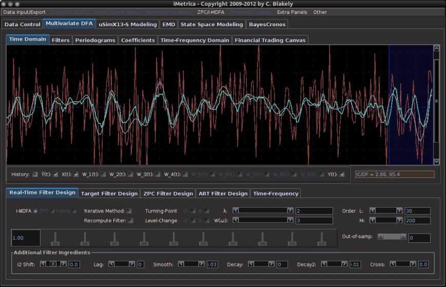
Figure 1. The original signal (green) built using 300 observations in-sample, and then applied to 30 out-of-sample observations. A high-order approximation to the target symmetric filter is plotted in gray. The blue shaded region is the region in which we wish to apply dynamic filter updating.

Now suppose we wish to improve performance of the signal in future out-of-sample observations by updating the filter coefficients to produce better smoothness, timeliness, and regularization properties. The first step is to ensure that the “Recompute Filter” option is not on (the checkbox in the Real-Time Filter Design panel. This should have been done already to produce the out-of-sample signal). Then go to the MDFA menu at the top of the software and click on “Adaptive Update”. This will pop open the Adaptive Filtering control panel from which we control everything in the new filter updating coefficients (see Figure 2).

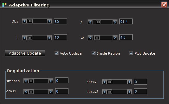
Figure 2. The panel interface for controlling every aspect of updating a filter in real-time.

The controls on the Adaptive Filtering panel are explained as follows:

• Obs. Sets the number of the latest observations used in the filter update. This is normally set to however many new observations out-of-sample have been streamed into the time series since the last filter computation. Although one can certainly include observations from the original in-sample period as well by simply setting Obs to a number higher than the number of recent out-of-sample observations. The minimum amount of observations is 10 and the maximum is the total length of the time series.
• L. Sets the length of the updating filter. Minimum is 5 and maximum is the number of observations minus 5.
• and . The customization of timeliness and smoothness parameters for the filter construction. These controls are strictly for the updating filter and independent of the ‘old’ filter.
• Adaptive Update. Once content with the settings of the update filter, press this button to compute the new filter and apply to the data. The results of the effects of the new filter will automatically appear in the main plotting canvas, specifically in the region of interest (shaded by blue, see blow).
• Auto Update. A check box that, if turned on, will automatically compute the new filter for any changes in the filter parameters and automatically plots the effects of the new filter in the main plotting canvas. This is a nice option to use when visually testing the output of the new filter as one can automatically see effects from any small changes to the parameter setting of the filter. This option also renders the “Adaptive Update” button obsolete.
• Shade Region. This check box, when activated, will shade the windowing region at the end of time series in which the updating is taking place. Provides a convenient way to pinpoint the exact region of interest for signal updating. The shaded region will appear in a dark blue shade (as shown in Figures 1, 4,6, and 7).
• Plot Updates. Clicking this checkbox on and off will plot the newly updated signal (on position) or the older signal (off position). This is a convenient feature as one is able to easily visually compare the new updated signal with the old signal to test for its effectiveness. If adding out-of-sample data and this feature is turned on, it will also apply the new updated filter coefficients to the new data as it comes in. If in the off position, it will only apply the ‘old’ filter coefficients.
• Regularization. All the regularization controls for the updating filter.

To update a signal in real-time, first select the number of observations and the length of the filter from the Obs and L sliding scrollbars, respectively. This will be the total number of observations used in the adaptive updating. For example, when new dynamics appear in the time series out-of-sample that the original old filter was not able to capture, the filter updating should include this new information.  Click the checkbox marked Shade Region to highlight in a dark shade of blue the region in which the updated signal will be computed (this is shown in Figure 1).  When the number of observations or length of filter changes, the shaded region reflects these changes and adjusts accordingly. After the region of interest is selected, customization and regularization of the signal can then be applied using the sliding scrollbars. Click the “Auto Update” checkbox to the ‘on’ position to see the effects of the parameterization on the signal computed in the highlighted region automatically. Once content with the filter parameterization, visually comparing the new updated signal with the old signal can be achieved simply by toggling the Plot Updates checkbox. To apply this new filter configuration to out-of-sample data, simply add more out-of-sample data by clicking the out-of-sample slider scrollbar control on the Real-Time Direct Filter control panel (provided that more out-of-sample data is available). This will automatically apply the ‘old’ original filter along with the updated filter on the new incoming out-of-sample data. If not content with the updated signal, simply remove the new out-of-sample data by clicking ‘back’ in the out-of-sample scrollbar, and adjust the parameters to your liking and try again. To continuously update the signal, simply reapply the above process as new out-of-sample data is added. As long as the “Plot Updates” is turned on, the newly adapted signal will always be plotted in the windowed region of interest. See Figures 4-7 to see this process in action.

In this example,  as previously mentioned, we computed the original signal in-sample using 300 observations and then applied the filter coefficients to 30 out-of-sample observations (this was produced by checking “Recompute Filter” off).  This is plotted in Figure 4, with the blue shaded region highlighting the 30 latest observations, our region of interest. Notice a significant mangling of timeliness and signal amplification in the pass-band of the filter. This is due to bad properties of the filter coefficients. Not enough regularization was applied. Surely enough, the amplitude of the frequency response function in the original filter shows the overshooting in the pass-band (see Figure 5).  To improve this signal, we apply an adaptive update by launching the Adaptive Update menu and configuring the new filter. Figure 6 shows the updated filter in the windowed region, where we chose a combination of timeliness and light regularization. There is a significant improvement in the timeliness of the signal. Any changes in the parameterization of the filter space is automatically computed and plotted on the canvas, a huge convenience as we can easily test different parameter configurations to easily identify the signal that satisfies the priorities of the user. In the final plot, Figure 7, we have chosen a configuration with a high amount of regularization to prevent overfitting. Compared with the previous two signals in the region of interest (Figures 4 and 6), we see an even greater mollification of the unwanted amplitude overshooting in the signal, without compromising with a lack of timeliness and smoothness properties. A high-order approximation to the targeted symmetric filter is also plotted in this example for comparison convenience (since the data is simulated, we know the future data, and hence the symmetric filter).

Tune in later this week for an example of Dynamic Adaptive Filtering applied to financial trading.

Figure 4. Plot of the signal out-of-sample before applying an update to the signal by allocating the 30 most recent out-of-sample observations and computing a new filter of length 10. The blue shaded region shows the updating region. Here the original old filter constructed in-sample has been applied to the 30 out-of-sample observations and we notice significant mangling of timeliness and signal amplification in the pass-band of the filter. This is due to bad properties of the filter coefficients. Not enough regularization was applied.

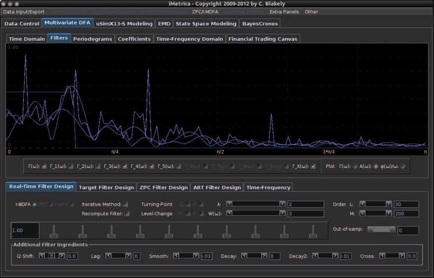
Figure 5. The overshooting in the pass-band of the frequency response function multivariate filter. The spikes above one in the pass-band indicate this and will most-likely produce overshooting in the signal out-of-sample.

Figure 6 After filter updating in the final 30 observations. We chose the filter settings in the adaptive filter settings to improve timeliness with a small amount of smoothing. Furthermore, regularization (smooth, decay) was applied to ensure no overfitting. Notice how the properties of the signal are vastly improved (namely timeliness and little to no overshooting).

Figure 7. Not satisfied with the results of our filter update, we can easily adjust the parameters more to find a satisfying configuration. In this example, since the data is simulated, I’ve computed the symmetric filter to compare my results with the theoretically “perfect” filter. After further adjusting regularization parameters, I end up with this signal shown in the plot. Here, the gray signal is a high-order approximation to the target symmetric “perfect” signal. The result is a very close fit to the target signal with no overfitting.