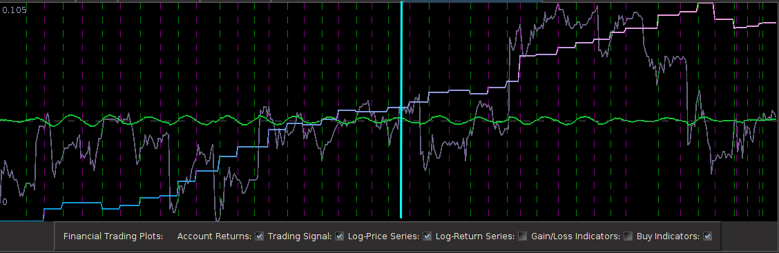
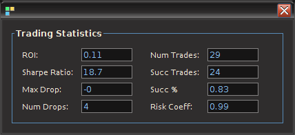
Figure 1: In-sample and Out-of-sample performance (observations 240-457) of the trading signal for the Euro Stoxx50 index futures with expiration March 18th (STXE H3) during the period of 1-9-2013 and 2-1-2013, using 15 minute log-returns. The black dotted lines indicate a buy/long signal and the blue dotted lines indicate a sell/short (top).
In this second tutorial on building high-frequency financial trading signals using the multivariate direct filter approach in R, I focus on the first example of my previous article on signal engineering in high-frequency trading of financial index futures where I consider 15-minute log-returns of the Euro STOXX50 index futures with expiration on March 18th, 2013 (STXE H3). As I mentioned in the introduction, I added a slightly new step in my approach to constructing the signals for intraday observations as I had been studying the problem of close-to-open variations in the frequency domain. With 15-minute log-return data, I look at the frequency structure related to the close-to-open variation in the price, namely when the price at close of market hours significantly differs from the price at open, an effect I’ve mentioned in my previous two articles dealing with intraday log-return data. I will show (this time in R) how MDFA can take advantage of this variation in price and profit from each one by ‘predicting’ with the extracted signal the jump or drop in the price at the open of the next trading day. Seems to good to be true, right? I demonstrate in this article how it’s possible.
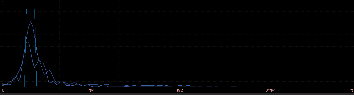
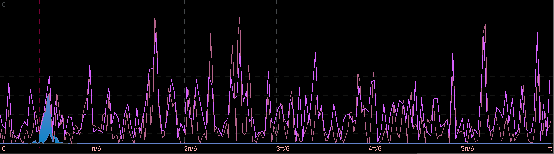
The first step after looking at the log-price and the log-return data of the asset being traded is to construct the periodogram of the in-sample data being traded on. In this example, I work with the same time frame I did with my previous R tutorial by considering the in-sample portion of my data to be from 1-4-2013 to 1-23-2013, with my out-of-sample data span being from 1-23-2013 to 2-1-2013, which will be used to analyze the true performance of the trading signal. The STXE data and the accompanying explanatory series of the EURO STOXX50 are first loaded into R and then the periodogram is computed as follows.
#load the log-return and log-price SXTE data in-sample
load(paste(path.pgm,"stxe_insamp15min.RData",sep=""))
load(paste(path.pgm,"stxe_priceinsamp15min.RData",sep=""))
#load the log-return and log-price SXTE data out-of-sample
load(paste(path.pgm,"stxe_outsamp15min.RData",sep=""))
load(paste(path.pgm,"stxe_priceoutsamp15min.RData",sep=""))

len_price<-557
out_samp_len<-210
in_samp_len<-347

price_insample<-stxeprice_insamp
price_outsample<-stxeprice_outsamp

#some mdfa definitions
x<-stxe_insamp
len<-length(x[,1])

#my range for the 15-min close-to-open cycle
cutoff<-.32
ub<-.32
lb<-.23

#------------ Compute DFTs ---------------------------
spec_obj<-spec_comp(len,x,0)
weight_func<-spec_obj$weight_func
stxe_periodogram<-abs(spec_obj$weight_func[,1])^2
K<-length(weight_func[,1])-1

#----------- compute Gamma ----------------------------
Gamma<-((0:K)<(K*ub/pi))&((0:K)>(K*lb/pi))

colo<-rainbow(6)
xaxis<-0:K*(pi/(K+1))
plot(xaxis, stxe_periodogram, main="Periodogram of STXE", xlab="Frequency", ylab="Periodogram",
xlim=c(0, 3.14), ylim=c(min(stxe_periodogram), max(stxe_periodogram)),col=colo[1],type="l" )
abline(v=c(ub,lb),col=4,lty=3)
You’ll notice in the periodogram of the in-sample STXE log-returns that I’ve pinpointed a spectral peak between two blue dashed lines. This peak corresponds to an intrinsically important cycle in the 15-minute log-returns of index futures that gives access to predicting the close-to-open variation in the price. As you’ll see, the cycle flows fluidly through the 26 15-minute intervals during each trading day and will cross zero at (usually) one to two points during each trading day to signal whether to go long or go short on the index for the next day. I’ve deduced this optimal frequency range in a prior analysis of this data that I did using my target filter toolkit in iMetrica (see previous article). This frequency range will depend on the frequency of intraday observations, and can also depend on the index (but in my experiments, this range is typically consistent to be between .23 and .32 for most index futures using 15min observations). Thus in the R code above, I’ve defined a frequency cutoff at .32 and upper and lower bandpass cutoffs at .32 and .23, respectively.

Figure 2: Periodogram of the log-return STXE data. The spectral peak is extracted and highlighted between the two red dashed lines.
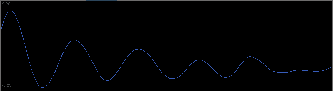
In this first part of the tutorial, I extract this cycle responsible for marking the close-to-open variations and show how well it can perform. As I’ve mentioned in my previous articles on trading signal extraction, I like to begin with the mean-square solution (i.e. no customization or regularization) to the extraction problem to see exactly what kind of parameterization I might need. To produce the plain vanilla mean-square solution, I set all the parameters to 0.0 and then compute the filter by calling the main MDFA function (shown below). The function IMDFA returns an object with the filter coefficients and the in-sample signal. It also plots the concurrent transfer function for both of the filters along with the filter coefficients for increasing lag, shown in Figure 3.
L<-86
lambda_smooth<-0.0
lambda_cross<-0.0
lambda_decay<-c(0.00,0.0)
i1<-F
i2<-F
lambda<-0
expweight<-0
i_mdfa_obj<-IMDFA(L,i1,i2,cutoff,lambda,expweight,lambda_cross,lambda_decay,lambda_smooth,weight_func,Gamma,x)
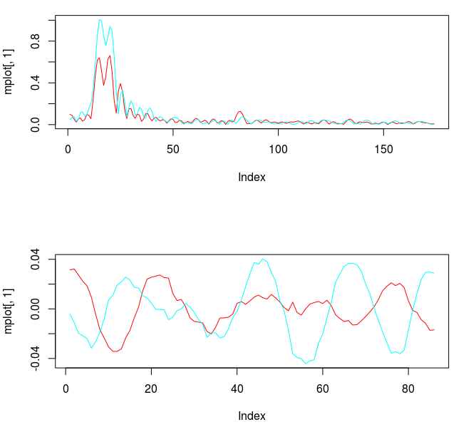
Figure 3: Concurrent transfer functions for the STXE (red) and explanatory series (cyan) (top). Coefficients for the STXE and explanatory series (bottom).
Notice the noise leakage past the stopband in the concurrent filter and the roughness of both sets of filter coefficients (due to overfitting). We would like to smooth both of these out, along with allowing the filter coefficients to decay as the lag increases. This ensures more consistent in-sample and out-of-sample properties of the filter. I first apply some smoothing to the stopband by applying an expweight parameter of 16, and to compensate slightly for this improved smoothness, I improve the timeliness by setting the lambda parameter to 1. After noticing the improvement in the smoothness of filter coefficients, I then proceed with the regularization and conclude with the following parameters.
lambda_smooth<-0.90
lambda_decay<-c(0.08,0.11)
lambda<-1
expweight<-16

Figure 4: Transfer functions and coefficients after smoothing and regularization.
A vast improvement over the mean-squared solution. Virtually no noise leakage in the stopband passed 
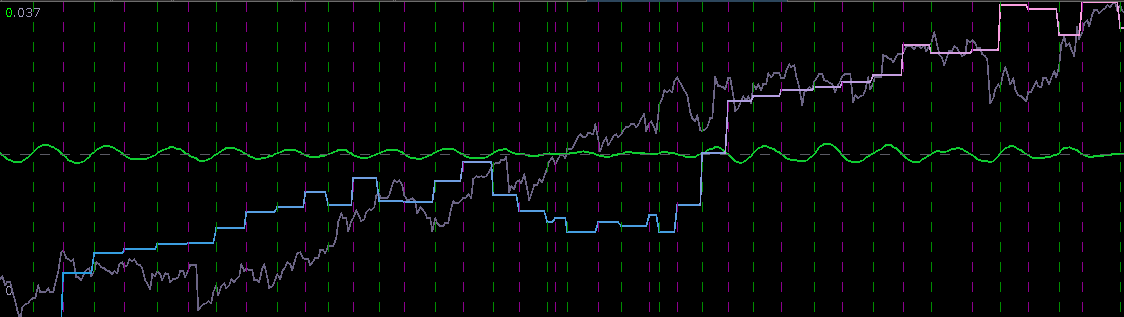
bn<-i_mdfa_obj$i_mdfa$b
trading_signal<-i_mdfa_obj$xff[,1] + i_mdfa_obj$xff[,2]

plot(x[L:len,1],col=colo[1],type="l")
lines(trading_signal[L:len],col=colo[4])
trade<-trading_logdiff(trading_signal[L:len],price_insample[L:len],0)

Figure 5: The in-sample signal and the log-returns of SXTE in 15 minute observations from 1-9-2013 to 1-23-2013
Figure 5 shows the log-return data and the trading signal extracted from the data. The spikes in the log-return data represent the close-to-open jumps in the STOXX Europe 50 index futures contract, occurring every 27 observations. But notice how regular the signal is, and how consistent this frequency range is found in the log-return data, almost like a perfect sinusoidal wave, with one complete cycle occurring nearly every 27 observations. This signal triggers trades that are shown in Figure 6, where the black dotted lines are buys/long and the blue dotted lines are sells/shorts. The signal is extremely consistent in finding the opportune times to buy and sell at the near optimal peaks, such as at observations 140, 197, and 240. It also ‘predicts’ the jump or fall of the EuroStoxx50 index future for the next trading day by triggering the necessary buy/sell signal, such as at observations 19, 40, 51, 99, 121, 156, and, 250. The performance of this trading in-sample is shown in Figure 7.

Figure 6: The in-sample trades. Black dotted lines are buy/long and the blue dotted lines are sell/short.
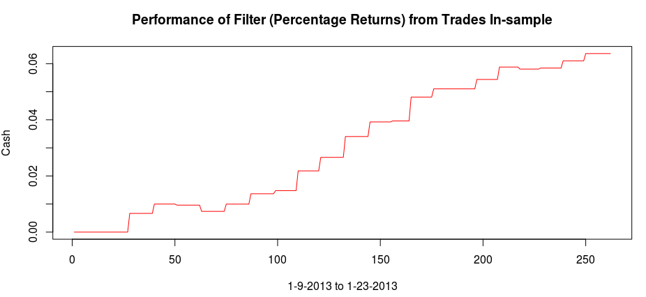
Figure 7: The in-sample performance of the trading signal.
Now for the real litmus test in the performance of this extracted signal, we need to apply the filter out-of-sample to check for consistency in not only performance, but also in trading characteristics. To do this in R, we bind the in-sample and out-of-sample data together and then apply the filter to the out-of-sample set (needing the final L-1 observations from the in-sample portion). The resulting signal in shown in Figure 8.
x_out<-rbind(stxe_insamp,stxe_outsamp)
xff<-matrix(nrow=out_samp_len,ncol=2)

  for(i in 1:out_samp_len)
  {
    xff[i,]<-0
    for(j in 2:3)
    {
      xff[i,j-1]<-xff[i,j-1]+bn[,j-1]%*%x_out[in_samp_len+i:(i-L+1),j]
    }
  }
  trading_signal_outsamp<-xff[,1] + xff[,2]

plot(stxe_outsamp[,1],col=colo[1],type="l")
lines(trading_signal_outsamp,col=colo[4])
The signal and log-return data Notice that the signal performs consistently out-of-sample until right around observation 170 when the log-returns become increasingly volatile. The intrinsic cycle between frequencies .23 and .32 has been slowed down due to this increased volatility and might affect the trading performance.

Figure 8: Signal produced out-of-sample on 210 observations and log-return data of STXE
The total in-sample plus out-of-sample trading performance is shown in Figure 9 and 10, with the final 210 points being out-of-sample. The out-of-sample performance is very much akin to the in-sample performance we had, with a very clear systematic trading exposed by ‘predicting’ the next day close-to-open jump or fall in a consistent manner, by triggering the necessary buy/sell signal, such as at observations 310, 363, 383, and 413, with only one loss up until the final day trading. The higher volatility during the final day of the in-sample period damages the cyclical signal and fails to trade systematically as it had been during the first 420 observations.
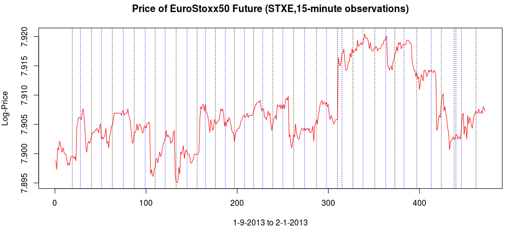
Figure 9: The total in-sample plus out-of-sample buys and sells.

Figure 10: Total performance over in-sample and out-of-sample periods.
With this kind of performance both in-sample and out-of-sample, and the beautifully consistent yet methodological trading patterns this signal provides, it would seem like attempting to improve upon it would be a pointless task. Why attempt to fix what’s not “broken”. But being the perfectionist that I am, I strive for an even “smarter” filter. If only there was a way to 1) keep the consistent cyclical trading effects as before 2) ‘predict’ the next day close-to-open jump/fall in the Euro Stoxx50 index future as before, and 3) avoid volatile periods to eliminate erroneous trading, where the signal performed worse. After hours spent in iMetrica, I figured how to do it. This is where advanced trading signal engineering comes into play.
The first step was to include all the lower frequencies below .23, which were not included in my previous trading signal. Due to the low amount of activity in these lower frequencies, this should only provide the effect or a ‘lift’ or a ‘push’ or the signal locally, while still retaining the cyclical component. So after changing my 

#---- set Gamma to low-pass
cutoff<-.32
Gamma<-((0:K)<(cutoff*K/pi))

#---- compute new filter ----------
i_mdfa_obj<-IMDFA(L,i1,i2,cutoff,lambda,expweight,lambda_cross,lambda_decay,lambda_smooth,weight_func,Gamma,x)

Figure 11: The concurrent transfer functions after changing to lowpass filter.
To improve the concurrent filter properties for both, I increase the smoothing expweight to 26, which will in turn affect the lambda_smooth, so I decrease it to .70. This gives me a much better transfer function pair, shown in Figure 12. Notice the peak in the explanatory series transfer function is now much closer to 1.0, exactly what we want.

Figure 12: The concurrent transfer functions after changing to lowpass filter, increasing expweight to 26, and decreasing lambda_smooth to .70.
I’m still not satisfied with the lift at frequency zero for the STXE series. At roughly .5 at frequency zero, the filter might not provide enough push or pull that I need. The only way to ensure a guaranteed lift in the STXE log-return series is to employ constraints on the filter coefficients so that the transfer function is one at frequency zero. This can be achieved by setting i1 to true in the IMDFA function call, which effectively ensures that the sum of the filter coefficients at 
#---- Update the regularization parameters
lambda_smooth<-0.68
lambda_cross<-0.0
lambda_decay<-c(0.083,0.11)

#---- update customization parameters
lambda<-0
expweight<-28

#---- set filter constraint -------
i1<-T
weight_constraint[1]<-1
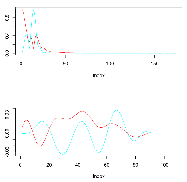
Figure 13: Transfer function and filter coefficients after setting the coefficient constraint i1 to true.
Now this is exactly what I was looking for. Not only does the transfer function for the explanatory series keep the important close-to-open cycle intact, but I have also enforced the lift I need for the STXE series. The coefficients still remain smooth with a nice decaying property at the end. With the new filter coefficients, I then applied them to the data both in-sample and out-of-sample, yielding the trading signal shown in Figure 14. It posses exactly the properties that I was seeking. The close-to-open cyclical component is still being extracted (thanks in part to the explanatory series), and is still relatively consistent, although not as much as the pure bandpass design. The feature that I like is the following: When the log-return data diverges away from the cyclical component, with increasing volatility, the STXE filter reacts by pushing the signal down to avoid any erroneous trading. This can be seen in observations 100 through 120 and then at observations 390 through the end of trading. Figure 15 (same as Figure 1 at the top of the article) show the resulting trades and performance produced in-sample and out-of-sample by this signal. This is the art of meticulous signal engineering folks.

Figure 14: In-sample and out-of-sample signal produced from the low-pass with i1 coefficient constraints.
With only two losses suffered out-of-sample during the roughly 9 days trading, the filter performs much more methodologically than before. Notice during the final two days trading, when volatility picked up, the signal ceases to trade as it is being pushed down. It even continues to ‘predict’ the close-to-open jump/fall correctly, such as at observations 288, 321, and 391. The last trade made was a sell/short sell position, with the signal trending down at the end. The filter is in position to make a huge gain from this timely signaling of a short position at 391, correctly determining a large fall the next trading day, and then waiting out the volatile trading. The gain should be large no matter what happens.

Figure 15: In-sample and out-of-sample performance of the i1 constrained filter design.
One thing I mention before concluding is that I made a slight adjustment to my filter design after employing the i1 constraint to get the results shown in Figure 13-15. I’ll leave this as an exercise for the reader to deduce what I have done. Hint: Look at the freezed degrees of freedom before and after applying the i1 constraint. If you still have trouble finding what I’ve done, email me and I’ll give you further hints.
Conclusion
The overall performance of the first filter built, in regards to total return on investment out-of-sample, was superior to the second. However, this superior performance comes only with the assumption that the cycle component defined between frequencies .23 and .32 will continue to be present in future observations of STXE up until the expiration. If volatility increases and this intrinsic cycle ceases to exist in the log-return data, the performance will deteriorate.
For a better more comfortable approach that deals with changing volatile index conditions, I would opt for ensuring that the local-bias is present in the signal, This will effectively push or pull the signal down or up when the intrinsic cycle is weak in the increasing volatility, resulting in a pullback in trading activity.
As before, you can acquire the high-freq data used in this tutorial by requesting it via email.
Happy extracting!


 . Once the bandpass target
  ,
,  , and
, and  .
.
 .
.
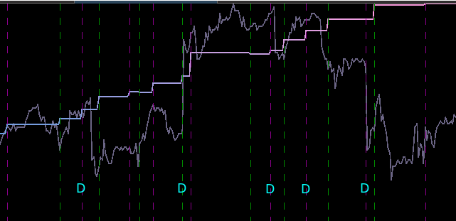
 from the band-pass design and setting the lower cutoff to 0. I also increased the smoothing parameter to $\alpha = 32$. In this newly designed filter, we see a vast improvement in the trading structure. As before, the filter was able to deduce the direction of every single close-to-open jump during the 200 out-of-sample observations, but notice that it was also able to become much more flexible in the trading during any upswing/downswing and volatile period. This is seen in more detail in Figure 7, where I added the letter ‘D’ to each of the 5 major buy/sell signals occurring before close.


 , down from
  as I had on the band-pass filter. This allows for slightly higher frequencies than

 , I then set the regularization parameters to be
  ,
,