MDFA-DeepLearning Package: Hybrid MDFA-RNN networks for machine learning in multivariate time series

Overview

MDFA-DeepLearning is a library for building machine learning applications on large numbers of multivariate time series data, with a heavy emphasis on noisy (non)stationary data.  The goal of MDFA-DeepLearning is to learn underlying patterns, signals, and regimes in multivariate time series and to detect, predict, or forecast them in real-time with the aid of both a real-time feature extraction system based on the multivariate direct filter approach (MDFA) and deep recurrent neural networks (RNN). The feature extraction system utilizes the MDFA-Toolkit to construct K multivariate signals in real-time (the features) where each of the K features targets a certain frequency range in the underlying time series.  Furthermore, each (or some) of these features can also be forecasted multiple steps ahead, or smoothed, creating many possibilities of signal or regime learning in time series.

For the deep learning components, in this package we focus on two network structures, namely a recurrent weighted average network (RWA  Ostmeyer and Cowell) and a standard long-short term memory network.  The RWA cell is a type of RNN cell that computes a recurrent weighted average over every past processing timestep, unlike standard RNN cells which only process information from previous timesteps.

The overall general architecture of the proposed network is given in Figure 1 in the case of an RWA network, which we will discuss in more detail below.  For a given sequence of N multivariate time series values which have been transformed appropriately to a stationary sequence, which we denote Y_1, Y_2, …, Y_N,  a real-time feature extraction process is applied at each observation which is then used as input to an RWA (or LSTM) network, where the univariate output is a targeted signal value (regression) or a regime value (classification)..

Selection_070.png

Figure 1: Proposed network design using RWA cells to learn form the real-time feature extractor. The Y_t values are the (multivariate) transformed time series values, and the S_t are univariate outputs describing a target signal or regime   

Why Use MDFA-DeepLearning

One might want to develop predictive models in multivariate time series data using MDFA-DeepLearning if the time series exhibit any of the following properties:

  • High-Dimensionality (many (un)correlated nonstationary time series)
  • Difficult to forecast using traditional model-based methods (VARIMA/GARCH) or traditional deep learning methods (RNN/LSTM, component decomposition, etc)
  • Emphasis needed on out-of-sample real-time signal extraction and forecasting
  • Regime changing in the underlying dynamics (or data generating process) of the time series is a common occurrence

The MDFA-DeepLearning approach differs from most machine learning methods in time series analysis in that an emphasis on real-time feature extraction is utilized where the features extractors are build using the multivariate direct filter approach. The motivation behind this coupling of MDFA with machine learning is that, while many time series decomposition methodologies exist (from empirical mode decomposition to stochastic component analysis methods), all of these rely on either in-sample decompositions on historical data (useless for future data), and/or assumptions about the boundary values, neither of which are attractive when fast, real-time out-of-sample predictions are the emphasis.  Furthermore, simply applying standard recurrent neural networks for step-ahead forecasting or signal extraction directly on the original noisy data is a useless exercise – the recurrent networks typically will only learn noise, producing signals and forecasts of little to no value (in most cases, the latter).

As mentioned, the back-end used for the novel feature extraction is the multivariate direct filter approach (MDFA), and is used to extract both local (higher-frequency) and global (low-frequency) features in real-time, out-of-sample, and output these features in a multivariate time series as inputs into an RWA or LSTM recurrent neural network. Thus the package is divided into essentially four different components which all need to be defined properly in order to produce predictive models for time series data:

  • Labeling interface
  • Feature extractors
  • DataSetIterator interface
  • Learning interface

Labeling interface

The package includes an interface for labeling time series. The labeling process takes segments of historical data, and labels each time series observation in some manner. There are three types of labels that can be used:

  • Observational labeling: every time series observation is labeled by a signal value (for example a target value computed by a symmetric target filter). This is sequence-to-sequence labeling for time series regression.
  • Fixed Period labeling: every period (day, week, etc) is labeled, typically by a one-hot vector. This is sequence-to-value labeling. The end of the period is labeled and the rest of the values are not (masked by nonvalues in the code).
  • Regime labeling: every value in a specific regime is labeled, either by a one-hot vector (for example, long (1,0) short (0,1) neutral (0,0), or trend (1,0) and mean-reverting (0,1)). This is another example of sequence-to-sequence, but using one-hot vectors and now in the form of sequence classification.

Other labeling strategies can certainly be used, but these are the three most common. We will give an outline on how to create a custom labeling strategy in a future article.

Feature Extractors

The package contains a feature extraction class called MDFAFeatureExtraction which, when instantiated, is used as the input to the a DataSetIterator. The MDFAFeatureExtraction contains a default automated feature extraction builder where a value of K is given as the number of features and a lag to indicate smoothing or forecasting steps-ahead.

One application of the MDFA feature extraction tool is to decompose a multivariate time series into K components in real-time which are close to being “orthogonal”, meaning in this sense that the frequency information from each of the components are relatively disjoint.  A precise mathematical formulation of this property and examples of the MDFAFeatureExtraction to follow.  Another example used for turning-point detection in trends is to decompose the multivariate series into K number of low-frequency components with different speeds and forecast/smoothing characteristics.

DataSetIterator

The DataSetIterator is an interface for ND4J that handles fast N-d array manipulation akin to numpy in Python. More specifically, the DataSetIterator handles traversing through a dataset and preparing data for a recurrent neural network. Our datasets in this package are outputs from the TimeSeries through the MDFAFeatureExtraction objects which then become the input to the RNN network. The DataSetIterator also performs the labeling and how output will be arranged. Thus it is essentially the communication from the underlying time series to the extraction process and then how it is treated as input and output to the RNN. In the package, we have designed two examples of DataSetIterators, one for regression and one for classification, that will be described in more detail in a later article.

Learning interface

Finally, the learning interface is where the final network is defined, all the parameters of the network, the activation and loss functions, and number/type of layers (LSTM, FeedForward, etc). The underlying computational framework for this component uses DeepLearning4J.

Requirements and Example

MDFA-DeepLearning requires both the MDFA-Toolkit package for constructing the time series feature extractors and the Eclipse Deeplearning4j (dl4j) library for the deep recurrent neural network constructors. The dl4j library is freely available at github.com/deeplearning4j, but is included in the build of this package using Gradle as the dependency management tool.

The back-end for the dl4j package will depend on your computational hardware, but is available on a local native basis using CPUs, or can take advantage of GPUs using CUDA libraries (CUDA 8.0 was used to test current version of MDFA-DeepLearnng). In this package I have included a reference to both versions (assuming a standard linux64 architecture).

The back-end used for the novel feature extraction technique, as mentioned, is the MDFA-Toolkit (available here), which will run on the ND4J package. The feature extraction begins by defining K MDFA objects, called MDFABase from the MDFA-Toolkit, with the fixed parameters set for each MDFA object. For example, here we define K=4 MDFABase objects, that will be used to extract different types of trends at different speeds in a fractionally differenced time series. Please refer to the MDFA-Toolkit documentation for more information on the definition of each MDFA parameter.

MDFABase[] anyMDFAs = new MDFABase[4];

anyMDFAs[0] = (new MDFABase()).setLowpassCutoff(Math.PI/8.0)
.setI1(1)
.setSmooth(.2)
.setLag(-3)
.setLambda(2.0)
.setAlpha(2.0)
.setFilterLength(5);

anyMDFAs[1] = (new MDFABase()).setLowpassCutoff(Math.PI/10.0)
.setLag(-2)
.setAlpha(2.0)
.setFilterLength(5);

anyMDFAs[2] = (new MDFABase()).setLowpassCutoff(Math.PI/4.0)
.setDecayStart(.1)
.setDecayStrength(.2)
.setLag(-1)
.setFilterLength(5);

anyMDFAs[3] = (new MDFABase()).setLowpassCutoff(Math.PI/14.0)
.setSmooth(.2)
.setDecayStart(.1)
.setDecayStrength(.1)
.setFilterLength(5);

More concrete, in-depth step by step examples and tutorials will be given in the source code on github and in this blog, but here we will just give a brief overview on an example main program using these features.


/* Define the .csv data file from where we built train/test dataIterators */
String[] dataFiles = new String[]{"AAPL.daily.csv"};

/* Information about the .csv timeseries file */
TimeSeriesFile fileInfo = new TimeSeriesFile("yyyy-MM-dd", "Index", "Open");

/* Define network parameters */
int miniBatchSize = 100;
int totalTrainExamples = 1500;
int totalTestExamples = 300;
int timeStepLength = 60;
int nHiddenLayers = 2;
int nHidden = 216;
int nEpochs = 400;
int seed = 123;
int iterations = 40;
double learningRate = .001;
double gradientNormThreshold = 10.0;

IUpdater updater = new Nesterovs(learningRate, .4);

/* Instantiate Feature Extractors as an array of MDFABase objects */
MDFAFeatureExtraction features = new MDFAFeatureExtraction(anyMDFAs); 

/* Instantiate a new RecurrentMdfaRegression network using the features defined above */
RecurrentMdfaRegression myNet = new RecurrentMdfaRegression(features);

/* Set the data and the DataIterator parameters */
myNet.setTrainingTestData(dataFiles, fileInfo, miniBatchSize, totalTrainExamples, totalTestExamples, timeStepLength);

/* Usually a good idea to normalize the data */
myNet.normalizeData();

/* Build the LSTM (default network) layers */
myNet.buildNetworkLayers(nHiddenLayers, nHidden,
			RecurrentMdfaRegression.setNeuralNetConfiguration(seed, iterations, learningRate, gradientNormThreshold, 0, updater));

/* An optional dl4j control panel to in the browser */
myNet.setupUserInterface();

/* Train on the number of Epochs */
myNet.train(nEpochs);

/* Print/plot results and stats */
myNet.printPredicitions();
myNet.plotBatches(10);

The main points here are that essentially three components need to be defined:

  1. The .csv time series data file from which the DataIterator will extract the time series data for both labeling and learning. Two data sets will be created from this, a train set and a test set. Referrencing to multiple files from which to extract training and test sets is also possible. In dl4j, training and test data is built in the form of a DataSetIterator interface (org.nd4j.linalg.dataset.api.iterator).  In the package, we have defined a MDFADataSetIterator and a MDFARegressionDataSetIterator. More DataSetIterators for various applications will be added on an ongoing basis.
  2. The network RecurrentMdfaRegression is initiated, and needs to contain the feature signal extractors. Any set of feature extractors can be added, here we used the ones defined above as an example.
  3. Finally, the LSTM (or recurrent weighted average) network parameters need to be defined, this will then be used to construct the layers of the recurrent network.

With these three steps defined the network should be ready to train and test. The challenge is of course defining the feature extraction parameters. In later articles, we will give tips and tricks into what works best for what type of learning applications in large time series.


Advertisement

MDFA-Toolkit: A JAVA package for real-time signal extraction in large multivariate time series

The multivariate direct filter approach (MDFA) is a generic real-time signal extraction and forecasting framework endowed with a richly parameterized interface allowing for adaptive and fully-regularized data analysis in large multivariate time series. The methodology is based primarily in the frequency domain, where all the optimization criteria is defined, from regularization, to forecasting, to filter constraints. For an in-depth tutorial on the mathematical formation, the reader is invited to check out any of the many publications or tutorials on the subject from blog.zhaw.ch.

This MDFA-Toolkit (clone here) provides a fast, modularized, and adaptive framework in JAVA for doing such real-time signal extraction for a variety of applications. Furthermore, we have developed several components to the package featuring streaming time series data analysis tools not known to be available anywhere else. Such new features include:

  • A fractional differencing optimization tool for transforming nonstationary time-series into stationary time series while preserving memory (inspired by Marcos Lopez de Prado’s recent book on Advances in Financial Machine Learning, Wiley 2018).
  • Easy to use interface to four different signal generation outputs:
    Univariate series -> univariate signal
    Univariate series -> multivariate signal
    Multivariate series -> univariate signal
    Multivariate series -> multivariate signal
  • Generalization of optimization criterion for the signal extraction. One can use a periodogram, or a model-based spectral density of the data, or anything in between.
  • Real-time adaptive parameterization control – make slight adjustments to the filter process parameterization effortlessly
  • Build a filtering process from simpler user-defined filters, applying customization and reducing degrees of freedom.

This package also provides an API to three other real-time data analysis frameworks that are now or soon available

  • iMetricaFX – An app written entirely in JavaFX for doing real-time time series data analysis with MDFA
  • MDFA-DeepLearning – A new recurrent neural network methodology for learning in large noisy time series
  • MDFA-Tradengineer – An automated algorithmic trading platform combining MDFA-Toolkit, MDFA-DeepLearning, and Esper – a library for complex event processing (CEP) and streaming analytics

To start the most basic signal extraction process using MDFA-Toolkit, three things need to be defined.

  1. The data streaming process which determines from where and what kind of data will be streamed
  2. A transformation of the data, which includes any logarithmic transform, normalization, and/or (fractional) differencing
  3. A signal extraction definition which is defined by the MDFA parameterization

Data streaming

In the current version, time series data is providing by a streaming CSVReader, where the time series index is given by a String DateTime stamp is the first column, and the value(s) are given in the following columns. For multivariate data, two options are available for streaming data.  1) A multiple column .csv file, with each value of the time series in a separate column 2) or in multiple referenced single column time-stamped .csv files. In this case, the time series DateTime stamps will be checked to see if in agreement. If not, an exception will be thrown. More sophisticated multivariate time series data streamers which account for missing values will soon be available.

Transforming the data

Depending on the type of time series data and the application or objectives of the real time signal extraction process, transforming the data in real-time might be an attractive feature. The transformation of the data can include (but not limited to) several different things

  • A Box-Cox transform, one of the more common transformations in financial and other non-stationary time series.
  • (fractional)-differencing, defined by a value d in [0,1]. When d=1, standard first-order differencing is applied.
  • For stationary series, standard mean-variance normalization or a more exotic GARCH normalization which attempts to model the underlying volatility is also available.

Signal extraction definition

Once the data streaming and transformation procedures have been defined, the signal extraction parameters can then be set in a univariate or multivariate setting. (Multiple signals can be constructed as well, so that the output is a multivariate signal. A signal extraction process can be defined by defining and MDFABase object (or an array of MDFABase objects in the mulivariate signal case). The parameters that are defined are as follows:

  • Filter length: the length L in number of lags of the resulting filter
  • Low-pass/band-pass frequency cutoffs: which frequency range is to be filtered from the time-series data
  • In-sample data length: how much historical data need to construct the MDFA filter
  • Customization: α (smoothness) and λ (timeliness) focuses on emphasizing smoothness of the filter by mollifying high-frequency noise and optimizing timeliness of filter by emphasizing error optimization in phase delay in frequency domain
  • Regularization parameters: controls the decay rate and strength, smoothness of the (multivariate) filter coefficients, and cross-series similarity in the multivariate case
  • Lag: controls the forecasting (negative values) or smoothing (positive values)
  • Filter constraints i1 and i2: Constrains the filter coefficients to sum to one (i1) and/or the dot product with (0,1…, L) is equal to the phase shift, where L is the filter length.
  • Phase-shift: the derivative of the frequency response function at the zero frequency.

All these parameters are controlled in an MDFABase object, which holds all the information associated with the filtering process. It includes it’s own interface which ensures the MDFA filter coefficients are updated automatically anytime the user changes a parameter in real-time.

Selection_069.png

Figure 1: Overview of the main module components of MDFA-Toolkit and how they are connected

As shown in Figure 1, the main components that need to be defined in order to define a signal extraction process in MDFA-Toolkit.  The signal extraction process begins with a handle on the data streaming process, which in this article we will demonstrate using a simple CSV market file reader that is included in the package. The CSV file should contain the raw time series data, and ideally a time (or date) stamp column. In the case there is no time stamp column, such a stamp will simply be made up for each value.

Once the data stream has been defined, these are then passed into a time series transformation process, which handles automatically all the data transformations which new data is streamed. As we’ll see, the TargetSeries object defines such transformations and all streaming data is passed added directly to the TargetSeries object. A MultivariateFXSeries is then initiated with references to each TargetSeries objects. The MDFABase objects contain the MDFA parameters and are added to the MultivariateFXSeries to produce the final signal extraction output.

To demonstrate these components and how they come together, we illustrate the package with a simple example where we wish to extract three independent signals from AAPL daily open prices from the past 5 years. We also do this in a multivariate setting, to see how all the components interact, yielding a multivariate series -> multivariate signal.


//Define three data source files, the first one will be the target series
String[] dataFiles = new String[]{"AAPL.daily.csv", "QQQ.daily.csv", "GOOG.daily.csv"};

//Create a CSV market feed, where Index is the Date column and Open is the data
CsvFeed marketFeed = new CsvFeed(dataFiles, "Index", "Open");

/* Create three independent signal extraction definitions using MDFABase:
One lowpass filter with cutoff PI/20 and two bandpass filters
*/
MDFABase[] anyMDFAs = new MDFABase[3];
anyMDFAs[0] = (new MDFABase()).setLowpassCutoff(Math.PI/20.0)
                              .setI1(1)
                              .setHybridForecast(.01)
                              .setSmooth(.3)
                              .setDecayStart(.1)
                              .setDecayStrength(.2)
                              .setLag(-2.0)
                              .setLambda(2.0)
                              .setAlpha(2.0)
                              .setSeriesLength(400); 

anyMDFAs[1] = (new MDFABase()).setLowpassCutoff(Math.PI/10.0)
                              .setBandPassCutoff(Math.PI/15.0)
                              .setSmooth(.1)
                              .setSeriesLength(400); 

anyMDFAs[2] = (new MDFABase()).setLowpassCutoff(Math.PI/5.0)
                              .setBandPassCutoff(Math.PI/10.0)
                              .setSmooth(.1)
                              .setSeriesLength(400);

/*
Instantiate a multivariate series, with the MDFABase definitions,
and the Date format of the CSV market feed
*/
MultivariateFXSeries fxSeries = new MultivariateFXSeries(anyMDFAs, "yyyy-MM-dd");

/*
Now add the three series, each one a TargetSeries representing the series
we will receive from the csv market feed. The TargetSeries
defines the data transformation. Here we use differencing order with
log-transform applied
*/
fxSeries.addSeries(new TargetSeries(1.0, true, "AAPL"));
fxSeries.addSeries(new TargetSeries(1.0, true, "QQQ"));
fxSeries.addSeries(new TargetSeries(1.0, true, "GOOG"));
/*
Now start filling the fxSeries will data, we will start with
600 of the first observations from the market feed
*/
for(int i = 0; i < 600; i++) {
   TimeSeriesEntry observation = marketFeed.getNextMultivariateObservation();
   fxSeries.addValue(observation.getDateTime(), observation.getValue());
}

//Now compute the filter coefficients with the current data
fxSeries.computeAllFilterCoefficients();

//You can also chop off some of the data, he we chop off 70 observations
fxSeries.chopFirstObservations(70);

//Plot the data so far
fxSeries.plotSignals("Original");

Selection_067.png

Figure 2: Output of the three signals on the target series (red) AAPL

In the first line, we reference three data sources (AAPL daily open, GOOG daily open, and SPY daily open), where all signals are constructed from the target signal which is by default, the first series referenced in the data market feed. The second two series act as explanatory series.  The filter coeffcients are computed using the latest 400 observations, since in this example 400 was used as the insample setSeriesLength, value for all signals. As a side note, different insample values can be used for each signal, which allows one to study the affects of insample data sizes on signal output quality.  Figure 2 shows the resulting insample signals created from the latest 400 observations.

We now add 600 more observations out-of-sample, chop off the first 400, and then see how one can change a couple of parameters on the first signal (first MDFABase object).


for(int i = 0; i < 600; i++) {
   TimeSeriesEntry observation = marketFeed.getNextMultivariateObservation();
   fxSeries.addValue(observation.getDateTime(), observation.getValue());
}

fxSeries.chopFirstObservations(400);
fxSeries.plotSignals("New 400");

/* Now change the lowpass cutoff to PI/6
   and the lag to -3.0 in the first signal (index 0) */
fxSeries.getMDFAFactory(0).setLowpassCutoff(Math.PI/6.0);
fxSeries.getMDFAFactory(0).setLag(-3.0);

/* Recompute the filter coefficients with new parameters */
fxSeries.computeFilterCoefficients(0);
fxSeries.plotSignals("Changed first signal");

Selection_067.png

Figure 3: After adding 600 new observations out-of-sample signal values

After adding the 600 values out-of-sample and plotting, we then proceed to change the lowpass cutoff of the first signal to PI/6, and the lag to -3.0 (forecasting three steps ahead). This is done by accessing the MDFAFactory and getting handle on first signal (index 0), and setting the new parameters. The filter coefficients are then recomputed on the newest 400 values (but now all signal values are insample).

In the MDFA-Toolkit, plotting is done using JFreeChart, however iMetricaFX provides an app for building signal extraction pipelines with this toolkit providing the backend where all the automated plotting, analysis, and graphics are handled in JavaFX, creating a much more interactive signal extraction environment. Many more features to the MDFA-Toolkit are being constantly added, especially in regard to features boosting applications in Machine Learning, such as we will see in the next upcoming article.

Big Data analytics in time series

We also implement in MDFA-Toolkit an interface to Apache Spark-TS, which provides a Spark RDD for Time series objects, geared towards high dimension multivariate time series. Large-scale time-series data shows up across a variety of domains. Distributed as the spark-ts package, a library developed by Cloudera’s Data Science team essentially enables analysis of data sets comprising millions of time series, each with millions of measurements. The Spark-TS package runs atop Apache Spark. A tutorial on creating an Apache Spark-TS connection with MDFA-Toolkit is currently being developed.

TWS-iMetrica: The Automated Intraday Financial Trading Interface Using Adaptive Multivariate Direct Filtering

Figure 1: The TWS-iMetrica automated financial trading platform. Featuring fast performance optimization, analysis, and trading design features unique to iMetrica for building direct real-time filters to generate automated trading signals for nearly any tradeable financial asset. The system was built using Java, C, and the Interactive Brokers IB API in Java.

Figure 1: The TWS-iMetrica automated financial trading platform. Featuring fast performance optimization, analysis, and trading design features unique to iMetrica for building direct real-time filters to generate automated trading signals for nearly any tradeable financial asset. The system was built using Java, C, and the Interactive Brokers IB API in Java.

Introduction

I realize that I’ve been MIA (missing in action for non-anglophones) the past three months on this blog, but I assure you there has been good reason for my long absence. Not only have I developed a large slew of various optimization, analysis, and statistical tools in iMetrica for constructing high-performance financial trading signals geared towards intraday trading which I will (slowly) be sharing over the next several months (with some of the secret-sauce-recipes kept to myself and my current clients of course), but I have also built, engineered, tested, and finally put into commission on a daily basis the planet’s first automated financial trading platform completely based on the recently developed FT-AMDFA (adaptive multivariate direct filtering approach for financial trading). I introduce to you iMetrica’s little sister, TWS-iMetrica.

Coupled with the original software I developed for hybrid econometrics, time series analysis, signal extraction, and multivariate direct filter engineering called iMetrica, the TWS-iMetrica platform was built in a way to provide an easy to use yet powerful, adaptive, versatile, and automated trading machine for intraday financial trading with a variety of options for building your own day trading strategies using MDFA based on your own financial priorities.  Being written completely in Java and gnu c, the TWS-iMetrica system currently uses the Interactive Brokers (IB) trading workstation (TWS) Java API in order to construct the automated trades, connect to the necessary historical data feeds, and provide a variety of tick data. Thus in order to run, the system will require an activated IB trading account. However, as I discuss in the conclusion of this article, the software was written in a way to be seamlessly adapted to any other brokerage/trading platform API, as long as the API is available in Java or has Java wrappers available.

The steps for setting up and building an intraday financial trading environment using iMetrica + TWS-iMetrica are easy. There are four of them. No technical analysis indicator garbage is used here, no time domain methodologies, or stochastic calculus. TWS-iMetrica is based completely on the frequency domain approach to building robust real-time multivariate filters that are designed to extract signals from tradable financial assets at any fixed observation of frequencies (the most commonly used in my trading experience with FT-AMDFA being 5, 15, 30, or 60 minute intervals). What makes this paradigm of financial trading versatile is the ability to construct trading signals based on your own trading priorities with each filter designed uniquely for a targeted asset to be traded. With that being said, the four main steps using both iMetrica and TWS-iMetrica are as follows:

  1. The first step to building an intraday trading environment is to construct what I call an MDFA portfolio (which I’ll define in a brief moment). This is achieved in the TWS-iMetrica interface that is endowed with a user-friendly portfolio construction panel shown below in Figure 4.
  2. With the desired MDFA portfolio, selected, one then proceeds in connecting TWS-iMetrica to IB by simply pressing the Connect button on the interface in order to download the historical data (see Figure 3).
  3. With the historical data saved, the iMetrica software is then used to upload the saved historical data and build the filters for the given portfolio using the MDFA module in iMetrica (see Figure 2). The filters are constructed using a sequence of proprietary MDFA optimization and analysis tools. Within the iMetrica MDFA module, three different types of filters can be built 1) a trend filter that extracts a fast moving trend 2) a band-pass filter for extracting local cycles, and 3) A multi-bandpass filter that extracts both a slow moving trend and local cycles simultaneously.
  4. Once the filters are constructed and saved in a file (a .cft file), the TWS-iMetrica system is ready to be used for intrady trading using the newly constructed and optimized filters (see Figure 6).
Figure 4: The iMetrica MDFA module for constructing the trading filters. Features dozens of design, analysis, and optimization components to fit the trading priorities of the user and is used in conjunction with the TWS-iMetrica interface.

Figure 2: The iMetrica MDFA module for constructing the trading filters. Features dozens of design, analysis, and optimization components to fit the trading priorities of the user and is used in conjunction with the TWS-iMetrica interface.

In the remaining part of this article, I give an overview of the main features of the TWS-iMetrica software and how easily one can create a high-performing automated trading strategy that fits the needs of the user.

The TWS-iMetrica Interface

The main TWS-iMetrica graphical user interface is composed of several components that allow for constructing a multitude of various MDFA intraday trading strategies, depending on one’s trading priorities. Figure 3 shows the layout of the GUI after first being launched. The first component is the top menu featuring TWS System, some basic TWS connection variables which, in most cases, these variables are left in their default mode, and the Portfolio menu. To access the main menu for setting up the MDFA trading environment, click Setup MDFA Portfolio under the Portfolio menu. Once this is clicked, a panel is displayed (shown in Figure 4) featuring the required a priori parameters for building the MDFA trading environment that should all be filled before MDFA filter construction and trading is to take place. The parameters and their possible values are given below Figure 4.

Figure 3 - The TWS-iMetrica interface when first launched and everything blank.

Figure 3 – The TWS-iMetrica interface when first launched and everything blank.

The Setup MDFA Portfolio panel featuring all the setting necessary to construct the automated trading MDFA environment.

Figure 4 – The Setup MDFA Portfolio panel featuring all the setting necessary to construct the automated trading MDFA environment.

  1. Portfolio – The portfolio is the basis for the MDFA trading platform and consists of two types of assets 1) The target asset from which we construct the trading signal, engineer the trades, and use in building the MDFA filter 2) The explanatory assets that provide the explanatory data for the target asset in the multivariate filter construction. Here, one can select up to four explanatory assets.
  2. Exchange – The exchange on which the assets are traded (according to IB).
  3. Asset Type – If the input portfolio is a selection of Stocks or Futures (Currencies and Options soon to be available).
  4. Expiration – If trading Futures, the expiration date of the contract, given as a six digit number of year then month (e.g. 201306 for June 2013).
  5. Shares/Contracts – The number of shares/contracts to trade (this number can also be changed throughout the trading day through the main panel).
  6. Observation frequency – In the MDFA financial trading method, we consider uniformly sampled observations of market data on which to do the trading (in seconds). The options are 1, 2, 3, 5, 15, 30, and 60 minute data. The default is 5 minutes.
  7. Data – For the intraday observations, determines the nature of data being extracted. Valid values include TRADES, MIDPOINT, BID, ASK, and BID_ASK. The default is MIDPOINT
  8. Historical Data – Selects how many days are used to for downloading the historical data to compute the initial MDFA filters. The historical data will of course come in intervals chosen in the observation frequency.

Once all the values have been set for the MDFA portfolio, click the Set and Build button which will first begin to check if the values entered are valid and if so, create the necessary data sets for TWS-iMetrica to initialize trading. This all must be done while TWS-iMetrica is connected to IB (not set in trading mode however). If the build was successful, the historical data of the desired target financial asset up to the most recent observation in regular market trading hours will be plotted on the graphics canvas. The historical data will be saved to a file named (by default) “lastSeriesData.dat” and the data will be come in columns, where the first column is the date/time of the observation, the second column is the price of the target asset, and remaining columns are log-returns of the target and explanatory data. And that’s it, the system is now setup to be used for financial trading. These values entered in the Setup MDFA Portfolio will never have to be set again (unless changes to the MDFA portfolio are needed of course).

Continuing on to the other controls and features of TWS-iMetrica, once the portfolio has been set, one can proceed to change any of the settings in main trading control panel. All these controls can be used/modified intraday while in automated MDFA trading mode. In the left most side of the panel at the main control panel (Figure 5) of the interface includes a set of options for the following features:

Figure 7 - The main control panel for choosing and/or modifying all the options during intraday trading.

Figure 5 – The main control panel for choosing and/or modifying all the options during intraday trading.

  1. In contracts/shares text field, one enters the amount of share (for stocks) or contracts (for futures)  that one will trade throughout the day. This can be adjusted during the day while the automated trading is activated, however, one must be certain that at the end of the day, the balance between bought and shorted contracts is zero, otherwise, you risk keeping contracts or shares overnight into the next trading day.Typically, this is set at the beginning before automated trading takes place and left alone.
  2. The data input file for loading historical data. The name of this file determines where the historical data associated with the MDFA portfolio constructed will be stored. This historical data will be needed in order to build the MDFA filters. By default this is “lastSeriesData.dat”. Usually this doesn’t need to be modified.
  3. The stop-loss activation and stop-loss slider bar, one can turn on/off the stop-loss and the stop-loss amount. This value determines how/where a stop-loss will be triggered relative to the price being bought/sold at and is completely dependent on the asset being traded.
  4. The interval search that determines how and when the trades will be made when the selected MDFA signal triggers a buy/sell transaction. If turned off, the transaction (a limit order determined by the bid/ask) will be made at the exact time that the buy/sell signal is triggered by the filter. If turned on, the value in the text field next to it gives how often (in seconds) the trade looks for a better price to make the transaction. This search runs until the next observation for the MDFA filter. For example, if 5 minute return data is being used to do the trading, the search looks every seconds for 5 minutes for a better price to make the given transaction. If at the end of the 5 minute period no better price has been found, the transaction is is made at the current ask/bid price. This feature has been shown to be quite useful during sideways or highly volatile markets.

The middle of the main control panel features the main buttons for both connecting to disconnecting from Interactive Brokers, initiating the MDFA automated trading environment, as well as convenient buttons used for instantaneous buy/sell triggers that supplement the automated system. It also features an on/off toggle button for activating the trades given in the MDFA automated trading environment. When checked on, transactions according to the automated MDFA environment will proceed and go through to the IB account. If turned off, the real-time market data feeds and historical data will continue to be read into the TWS-iMetrica system and the signals according to the filters will be automatically computed, but no actual transactions/trades into the IB account will be made.

Finally, on the right hand side of the main control panel features the filter uploading and selection boxes. These are the MDFA filters that are constructed using the MDFA module in iMetrica. One convenient and useful feature of TWS-iMetrica is the ability to utilize up to three direct real-time filters in parallel and to switch at any given moment during market hours between the filters. (Such a feature enhances the adaptability of the trading using MDFA filters. I’ll discuss more about this in further detail shortly).  In order to select up to three filters simultaneously, there is a filter selection panel (shown in bottom right corner of Figure 6 below) displaying three separate file choosers and a radio button corresponding to each filter. Clicking on the filter load button produces a file dialog box from which one selects a filter (a *.cft file produced by iMetrica). Once the filter is loaded properly, on success, the name of the filter is displayed in the text box to the right, and the radio button to the left is enabled. With multiple filters loaded, to select between any of them, simply click on their respective radio button and the corresponding signal will be plotted on the plot canvas (assuming market data has been loaded into the TWS-iMetrica using the market data file upload and/or has been connected to the IB TWS for live market data feeds). This is shown in Figure 6.

Figure 5 - The TWS-iMetrica main trading interface features many control options to design your own automated MDFA trading strategies.

Figure 6 – The TWS-iMetrica main trading interface features many control options to design your own automated MDFA trading strategies.

And finally, once the historical data file for the MDFA portfolio has been created, up to three filters have been created for the portfolio and entered in the filter selection boxes, and the system is connected to Interactive Brokers by pressing the Connect button, the market and signal plot panel can then be used for visualizing the different components that one will need for analyzing the market, signal, and performance of the automated trading environment. In the panel just below the plot canvas features and array of checkboxes and radiobuttons. When connected to IB and the Start MDFA Trading has been pressed, all the data and plots are updated in real-time automatically at the specific observation frequency selected in the MDFA Portfolio setup. The currently available plots are as follows:

Figure 8 - The plots for the trading interface. Features price, log-return, account cumulative returns, signal, buy/sell lines, and up to two additional  auxiliary signals.

Figure 8 – The plots for the trading interface. Features price, log-return, account cumulative returns, signal, buy/sell lines, and up to two additional auxiliary signals.

  • Price – Plots in real-time the price of the asset being traded, at the specific observation frequency selected for the MDFA portfolio.
  • Log-returns – Plots in real-time the log-returns of the price, which is the data that is being filtered to construct the trading signal.
  • Account – Shows the cumulative returns produced by the currently chosen MDFA filter over the current and historical data period (note that this does not necessary reflect the actual returns made by the strategy in IB, just the theoretical returns over time if this particular filter had been used).
  • Buy/Sell lines – Shows dashed lines where the MDFA trading signal has produced a buy/sell transaction. The green lines are the buy signals (entered a long position) and magenta lines are the sell (entered a short position).
  • Signal – The plot of the signal in real-time. When new data becomes available, the signal is automatically computed and replotted in real-time. This gives one the ability to closely monitory how the current filter is reacting to the incoming data.
  • Aux Signal 1/2 – (If available) Plots of the other available signals produced by the (up to two) other filters constructed and entered in the system. To make either of these auxillary signals the main trading signal simply select the filter associated with the signal using the radio buttons in the filter selection panel.

Along with these plots, to track specific values of any of these plots at anytime, select the desired plot in the Track Plot region of the panel bar. Once selected, specific values and their respective times/dates are displayed in the upper left corner of the plot panel by simply placing the mouse cursor over the plot panel. A small tracking ball will then be moved along the specific plot in accordance with movements by the mouse cursor.

With the graphics panel displaying the performance in real-time of each filter, one can seamlessly switch between a band-pass filter or a timely trend (low-pass) filter according to the changing intraday market conditions. To give an example, suppose at early morning trading hours there is an unusual high amount of volume pushing an uptrend or pulling a downtrend. In such conditions a trend filter is much more appropriate, being able to follow the large-variation in log-returns much better than a band-pass filter can. One can glean from the effects of the trend filter on the morning hours of the market. After automated trading using the trend filter, with the volume diffusing into the noon hour, the band-pass filter can then be applied in order to extract and trade at certain low frequency cycles in the log-return data. Towards the end of the day, with volume continuously picking up, the trend filter can then be selected again in order to track and trade any trending movement automatically.

I am in the process of currently building an automated algorithm to “intelligently” switch between the uploaded filters according to the instantaneous market conditions (with triggering of the switching being set by volume and volatility. Otherwise, for the time being, currently the user must manually switch between different filters, if such switching is at all desired (in most cases, I prefer to leave one filter running all day. Since the process is automated, I prefer to have minimal (if any) interaction with the software during the day while it’s in automated trading mode).

Conclusion

As I mentioned earlier, the main components of the TWS-iMetrica were written in a way to be adaptable to other brokerage/trading APIs. The only major condition is that the API either be available in Java, or at least have (possibly third-party?) wrappers available in Java. That being said, there are only three main types of general calls that are made automated to the connected broker 1) retrieve historical data for any asset(s), at any given time, at most commonly used observation frequencies (e.g. 1 min, 5 min, 10 min, etc.), 2) subscribe to automatic feed of bar/tick data to retrieve latest OHLC and bid/ask data, and finally 3) Place an order (buy/sell) to the broker with different any order conditions (limit, stop-loss, market order, etc.) for any given asset.

If you are interested in having TWS-iMetrica be built for your particular brokerage/trading platform (other than IB of course) and the above conditions for the API are met, I am more than happy to be hired at certain fixed compensation, simply get in contact with me. If you are interested seeing how well the automated system has performed thus far, interested in future collaboration, or becoming a client in order to use the TWS-iMetrica platform, feel free to contact me as well.

Happy extracting!

Dream within a dream: How science fiction concepts from the movie Inception can be accomplished in real life (via MDFA)

“Careful, we may be in a model…within a model.” (From an Inception movie poster.)

“Careful, we may be in a model…within a model.” (From an Inception movie poster.)

Have you ever seen the movie Inception and wondered, “Gee, wouldn’t it be neat if I could do all that fancy subconscious dream within a dream manipulation stuff”? Well now you can (in a metaphorical way) using MDFA and iMetrica. I explain how in this article.

Before I begin, may I first draw your attention to a brief introduction of the context in which I am speaking, and that is real-time signal extraction in (nonlinear, nonstationary) information flow. The principle goal of filtering and signal extraction in real-time data analysis for whatever purpose necessary (financial trading, risk analysis, real-time trend detection, seasonal adjustment) is to detect and pinpoint as timely as possible a desired sequence of events in an incoming flow of data observations. We emphasize that this detection should be fast, in that the desired signal, or sequence of events, should be so robust in its timeliness and accuracy so as to detect turning points or actions in targeted events as they happen, or even become so awesome that it manages to anticipate what will happen in the future. Of course, this is never an exact science nor even always possible (otherwise we’d all be billionaires right?) and thus we rely on creative ways to cope with the unknown.

We can also think of signal extraction in more abstract terms. Real-time signal extraction entails the construction of a ‘smart’ illusion, an alternative to reality, where reality in this context is a time series, the information flow, the raw data. This ‘smart’ illusion that is being constructed is the signal, the vital information that has been extracted from an abundance of “noise” embedded in the reality. And the signal must produce important underlying secrets to satisfy the needs of the user, the signal extractor. How these signals are extracted from reality is the grand challenge. How are they produced in a robust, fast, and feasible manner so as to be effective in the real-time flow of information? The answer is in MDFA, or in other words as I’ll describe in this article, penetrating the subconscious state of reality to gain access to hidden treasures.

After recently re-watching the Christopher Nolan opus entitled Inception starring Leonardo DiCaprio and what seems like most of the cast from the Dark Knight Trilogy, I began to see some similarities between the main concepts entertainingly presented in the movie (using some pimped-up CGI), and the mathematics of  signal extraction using the multivariate direct filtering approach (MDFA). In this article I present some of these interesting parallels that I’ve managed to weave together.  My ultimate goal with this article is to hopefully paint a vivid picture of some interesting details stemming from the mathematics of the direct filtering approach by using the parallels that I’ve contrived between the two. Afterwards, hopefully you’ll be on your way to entering the realm of ‘dreaming within dreaming’, and extracting pertinent hidden secrets embedded in a flurry of noise.

The film introduces a slick con man by the name of Cobb (played by DiCaprio), and his team of super well-dressed con artists with leather jackets and slicked back hair (the classic con man look right?). The catchy idea that resides in the premise of the film is that these aren’t ordinary con men: they have a unique way of manipulating reality: by entering the dreams (subconscious ) of their targets (or marks as they call them in the film) and manipulate their subconscious dream state under the goal of extracting a desired idea or hidden secret. Like any group of con men, they attempt to construct a false reality by creating a certain architecture and environment in the target’s dream. The effectiveness of this ‘heist’ to capture the desired signals in the dream relies on the quality of the architecture and environment of the dream.

So how does all this relate to the mathematics of the MDFA for signal extraction. My vision can be seen as follows. In manipulating the target’s subconscious , Cobb’s group basically involves a collection of four components. Each one can be associated with a mathematical concept embedded in the MDFA.

The Target – At the highest level, we have reality. The real world in which the characters, and the target (victim), live. The target victim has an abundance of hidden information among the large capacity of mostly noise, from which Cobb’s group wish to manipulate and extract a hidden secret, the signal. In the MDFA world, we can associate or represent the information flow, the time series on which we perform the signal extraction process as the target victim in the real world. This is the data that we see, the reality. This data of course is non-deterministic,  namely we have no idea what the target victim has in mind for the future. The process of extracting the hidden thoughts or ideas from this target victim is akin to, in the MDFA world, the signal extraction process. The tools used to do the extracting are as follows.

The Extractor – The extractor is depicted in Inception as a master con man, a person who knows how to manipulate a subject (the target) in their subconscious dreaming world into revealing their deepest mental secrets. As the extractor’s goal is manipulation of the subconscious of a target to reveal a certain signal buried within reality, the extractor must transform the real-world conscious mental state of the target from reality into the dreaming subconscious world, by inducing a dream state. The multivariate direct filtering process of transforming the data (reality) into spectral frequency space (the subconscious ) via the Fourier transform to reveal the signal given the desired target data is metaphorically very similar to this process. The Inception extractor can be seen as being parallel to the process of transforming the data from reality into a subconscious world, the spectral frequency domain. It’s in this dreaming subconscious world, the frequency domain, where the real manipulation begins, using an architect.

The Architect – The Inception architect is the designer of the dream who constructs and builds the subconscious world into which the extractor brings the subject, or target. Just as the architect manipulates real world architecture and physics in order to create paradoxes like an endless staircase, folding buildings, smooth transitions from one place to another and other various phenomena otherwise impossible in the real world, the architect in the filtering world is the toolkit of filtering parameters that render the finite-dimensional metric space in which one constructs the filter coefficients to produce the desired signal. This includes the extraction rules (namely the symmetric target filter), customization for timeliness and speed, and regularization to warp and bend the finite dimensional filter metric space. Just as many different paths in the subconscious world toward the manipulation of the target subject exist and it is the architect’s job to create the optimal environment for extracting the desired signal, the architect in the direct filtering world uses the wide ranging set of filter parameters to bend and manipulate the metric space from which the filter coefficients are built and then used in the signal extraction process. Just as changing dynamics in the Inception real world (like the state of free-falling) will change the physics of the dreamt subconscious world (like floating in hotel elevator shafts while engaging in physical combat, Matrix style),  changing dynamics in the information flow will alter the geometry of the consequent architecture being built for the filter. And furthermore, just as the dream architect must be highly skilled in order to manipulate correctly, the MDFA architect must be highly skilled in order to construct the appropriate space in which the optimal signal is extracted (hint hint, call me or Marc, we’re the extractors and architects).

Dream within a dream – As one of the more fascinating concepts introduced in Inception, the concept of the dream within a dream was also the main trick to their success in dream manipulation. Starting from reality, each level of the dreaming subconscious state can be further transposed into another level of subconscious , namely dreaming within a dream. The dream within a dream process puts you into a deeper state of dreaming. The deeper you go, the further one’s mind is removed from reality. This is where the subject of dynamic adaptive filtering comes into play (see my previous article here for an intro and basics to dynamic adaptive filtering in iMetrica). In the direct filtering world, dynamic adaptive filtering is akin to the dream within a dream concept: Once in a level of subconscious (the spectral frequency space in MDFA), and the architect has created the dream used for manipulation (the metric space for the filter coefficients), a new level of subconscious can then be entered by introducing a newly adapted metric space based on the information extracted from the first level of subconscious.

In the dream within a dream, time is the other factor. The deeper you go into a dream state, the faster your mind is able to imagine and perceive things within that dream state. For example, one minute in reality can seem like one hour in the dream state. At the next level of subconscious, at each level in the subconscious , the element of time speeds up exponentially. A similar analogy can be extracted (no pun intended) in the concept of dynamic adaptive filtering. In dynamic adaptive filtering, we first begin by extracting a signal with the desired filter architecture at the first level transformation from reality to the spectral frequency space. When new information is received and our extracted signal is not behaving how we desire, we can build a new filter architecture for manipulating the signal with the newly provided information, with all the filter parameters available to control the desired filter properties. We are inherently building a new updated filter architecture on top of the old filter architecture, and consequently building a new signal from the output of the old signal by correcting (manipulating) this old signal toward our desired goals. This is akin to the dream within a dream concept. And just like the idea of time passing much faster at each subconscious level, the effects of filter parameters for controlling regularization and speed occur at a much faster rate since we are dealing with less information, a much shorter time frame (namely the newly arrived information) at each subsequent filtering level. One can even continue down the levels of subconscious, building a new architecture on top of the previous architecture, continuously using the newly provided information at each level to build the next level of subconsciousness; dream within a dream within a dream.

To summarize these analogies, I’ll be adding a graphic soon to this article that explains in a more succinct manner these parallels described above between Inception and MDFA. In the meantime, here are the temporary replacements.

Haters gonna hate... extractors gonna extract.

Haters gonna hate… extractors gonna extract.

Nolan, why you leavin' Leo out?

Nolan, why you leavin’ Leo out?

Dynamic Adaptive Filtering and Signal Extraction

This slideshow requires JavaScript.

Introduction

Dynamic adaptive filtering is the method of updating a signal extraction process in real-time using newly provided information. This newly provided information is the next sequence of observed data, such as minute, hourly, or daily log-returns in a portfolio of financial assets, or a new set of weekly/monthly observations in a set of economic indicators. The goal is to improve the properties of the extracted signal with respect to a target (symmetric) filter and the output of past (old) signal values that are not performing as they should be (perhaps due to overfitting). In the multivariate direct filtering approach framework, it is an easily workable task to update the signal while only using the most recent information given. As a recently proposed idea by Marc Wildi last month, in this dynamic form of adaptive filtering we seek to update and improve a signal for a given multivariate time series information flow by computing a new set of filter coefficients to only a small window of the time series that features the latest observations. Instead of recomputing an entire new set of filter coefficients in-sample on the entire data set, we use a much smaller data set, say the latest \tilde{N} observations on which the older filter was applied out-of-sample which is much less than the total number of observations in the time series.

The new filter coefficients computed on this small window of new observations uses as input the filtered series from original ‘old’ filter. These new updated coefficients are then applied to the output of the old filter, leading to completely re-optimized filter coefficients and thus an optimized signal, eliminating any nasty effects due overfitting or signal ‘overshooting’ in the older filter, while at the same time utilizing new information. This approach is akin to, in a way, filtering within filtering: the idea of ‘smart’-filtering on previously filtered data for optimized control of the new signal being computed. It could also be thought of as filtering filtered data, a convolution of filters, updating the real-time signal, or, more generally, adaptive filtering. However you wish to think of it, the idea is that a new filter provides the necessary updating by correcting the signal output of the old filter, applied to data out-of-sample. A rather smart idea as we will see. With the coefficients of the old filter are kept fixed, we enter into the frequency world of the output of the ‘old’ filter to gain information on optimizing the new filter. Only the coefficients of the new updated filter are optimized, and can be optimized anytime new data becomes available. This adaptive process is dynamic in the sense that we require new information to stream in in order to update the new signal by constructing a new filter. Once the new filter is constructed, the newly adapted signal is built by first applying the old filter to the data to produce the initial (non-updated) signal from the new data, then the newly constructed filter optimized from this output is then applied to the ‘old’ signal producing the smarter updated signal. Below is an outline of this algorithm for dynamic adaptive filtering stripped of much of the mathematical details. A more in-depth look at the mathematical details of MDFA and this newly proposed adaptive filtering method can be found in section 10.1 of the Elements paper by Wildi.

Basic Algorithm

We begin with a target time series Y_t, t=1,\ldots, N from which we wish to extract a signal, and along with it a set of M explanatory time series Y_{j,t}, t=1,\ldots,N, j=1,\ldots,M that may help in describing the dynamics of our target time series Y_t. Note that in many applications, such as financial trading, we normally set Y_{1,t} = Y_t so that our target time series is included in the explanatory time series set, which makes sense since it is the only known time series to perfectly describe itself (however, not in every signal extraction applications is this a good idea. See for example the GDP filtering work of Wildi here)To extract the initial signal in the given data set (in-sample), we define a target filter \Gamma(\omega), that lives on the frequency domain \omega \in [0,\pi]. We define the architecture of the filter metric space for the initial signal extraction by the set of parameters \Theta_0 := (L, \Gamma, \alpha, \lambda, i1, i2, \lambda_{s}, \lambda_{d}, \lambda{c}), where L is the desired length of the filter, \alpha and \lambda are the smoothness and timeliness customization controls, and \lambda_{s}, \lambda_{d}, \lambda{c} are the regularization parameters for smooth, decay, and cross, respectively. Once the filter is computed, we obtain a collection of filter coefficients b^j_l, l=0,\ldots,L-1 for each explanatory time series j=1,\ldots,M. The in-sample real-time signal X_t, t = L-1,\ldots,N is then produced by applying the filter coefficients on each respective explanatory series.

Now suppose we have new information flowing. With each new observation in our explanatory series Y_{j,t}, t=N+1,\ldots, we can apply the filter coefficients b^j_l to obtain the extracted signal X_t for the real-time estimate of the desired signal at each new observation t=N+1,\ldots. This is, of course, out-of-sample signal extraction. With the new information available from say t=N+1 to t=N+\tilde{N}, we wish to update our signal to include this new information. Instead of recomputing the entire filter for the N+\tilde{N}, a smarter idea recently proposed last month by Wildi in his MDFA blog is to use the output produced by applying each individual filter coefficient set b^j_l on their respective explanatory series as input into building the newly updated filter X_{j,t} = \sum_{l=0}^L b^j_l Y_{j,t-l}. We thus create a new set of M time series X_{j,t}, t=N+1,\ldots,\tilde{N} and thus the filtered explanatory data series become the input to the MDFA solver, where we now solve for a new set of filter coefficients b^j_{l,new} to be applied on the output of the old filter of the new incoming data. In this new filter construction, we build a new architecture for the signal extraction, where a whole new set of parameters can be used \Theta_1 := (L_1, \Gamma, \tilde{\alpha}, \tilde{\lambda}, i1, i2, \tilde{\lambda}_{s}, \tilde{\lambda}_{d}, \tilde{\lambda}_{c}). This is the main idea behind this dynamic adaptive filtering process: we are building a signal extraction architecture within another signal extraction architecture since we are basing this new update design on previous signal extraction performance.  Furthermore, since a much shorter span of observations, namely \tilde{N} << N
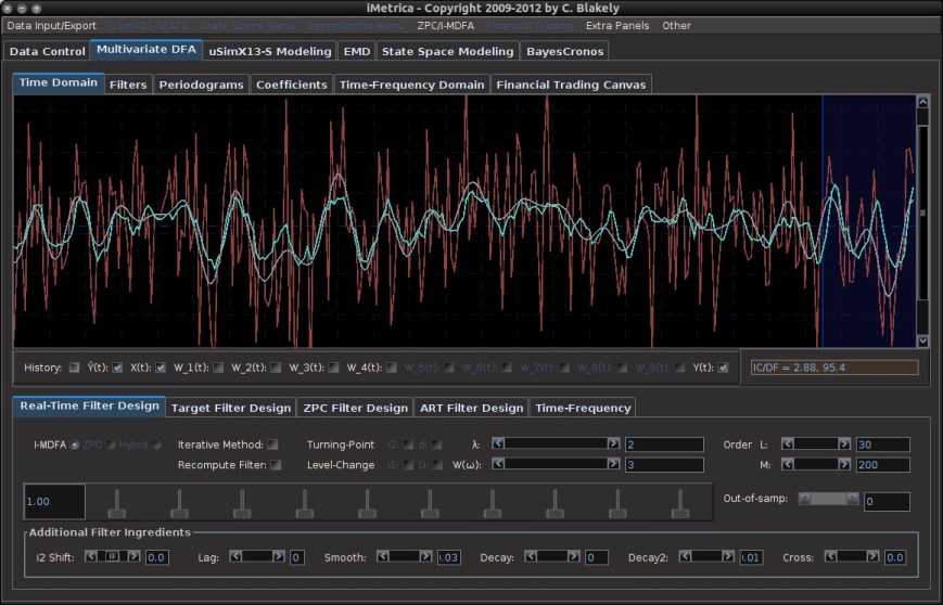
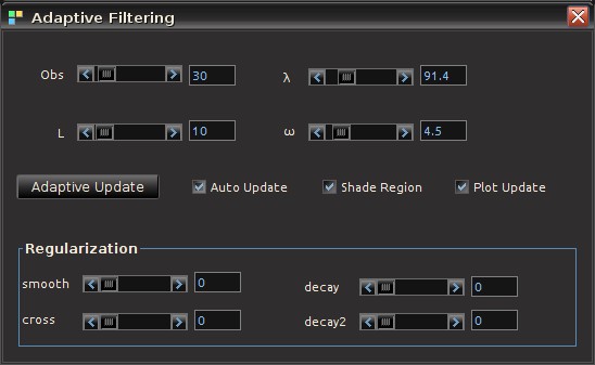
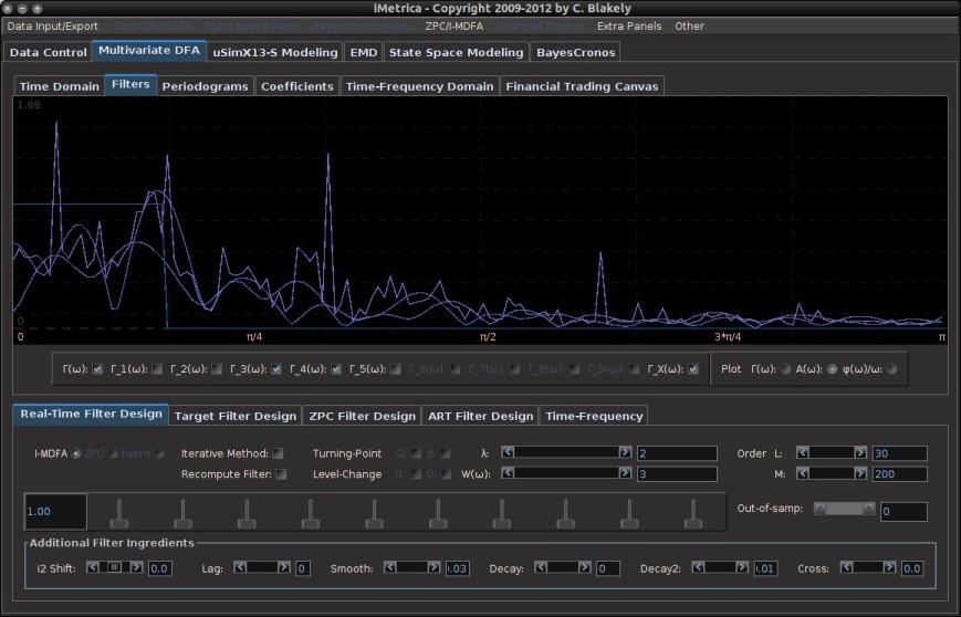
, is being used to construct the new filters, one of the advantages of this filter updating is that it is extremely fast, as well as being effective. As we will show in the next section of this article, all aspects of this dynamic adaptive filtering can be easily controlled, tested, and applied in the MDFA module of iMetrica using a new adaptive filtering control panel. One can control all aspects, from filter length to all the filter parameters in the new updated filter design, and then apply the results to out-of-sample data to compare performance.

Dynamic Adaptive Filtering Interface in iMetrica

The adaptive filtering capabilities in iMetrica are controlled by an interface that allows for adjusting all aspects of the adaptive filter, including number of observations, filter length L, customization controls for timeliness and smoothness, and controls for regularization. The process for controlling and applying dynamic adaptive filtering in iMetrica is accomplished as follows. Firstly, the following two things are required in order to perform dynamic adaptive filtering.

  1. Data. A target time series and (optional) M explanatory series that describe the target series all available on N observations for in-sample filter computation along with a stream of future information flow (i.e. an additional set of, say \tilde{N}, future observations for each of the M + 1 series.
  2. An initial set of optimized filter coefficients b^j_l for the signal of the data in-sample.

With these two prerequisites, we are now ready to test different dynamic adaptive filtering strategies. Figure 1 shows the MDFA module interface with time series data of a target series (shown in red) and four explanatory series (not plotted). Using the parameter configuration shown in Figure 1, an initial filter for computing the signal (green plot) that has been optimized in-sample on 300 observations of data and then applied to 30 out-of-sample observations (shown in the blue shaded region). As these final 30 observations of the signal have been produced using 30 out-of-sample observations, we can take note of its out-of-sample performance. Here, the performance of the signal has much room to improve. In this example, we use simulated data (conditionally heteroskedastic data generating process to emulate log-return type data) so that we are able to compare the computed updated signals with a high-order approximation of the target symmetric “perfect” signal (shown in gray in Figure 1).

The original signal (green) built using 300 observations in-sample, and then applied to 30 out-of-sample observations. A high-order approximation to the target symmetric filter is plotted in gray.

Figure 1. The original signal (green) built using 300 observations in-sample, and then applied to 30 out-of-sample observations. A high-order approximation to the target symmetric filter is plotted in gray. The blue shaded region is the region in which we wish to apply dynamic filter updating.

Now suppose we wish to improve performance of the signal in future out-of-sample observations by updating the filter coefficients to produce better smoothness, timeliness, and regularization properties. The first step is to ensure that the “Recompute Filter” option is not on (the checkbox in the Real-Time Filter Design panel. This should have been done already to produce the out-of-sample signal). Then go to the MDFA menu at the top of the software and click on “Adaptive Update”. This will pop open the Adaptive Filtering control panel from which we control everything in the new filter updating coefficients (see Figure 2).

The panel interface for controlling every aspect of updating a filter.

Figure 2. The panel interface for controlling every aspect of updating a filter in real-time.

The controls on the Adaptive Filtering panel are explained as follows:

  • Obs. Sets the number of the latest observations used in the filter update. This is normally set to however many new observations out-of-sample have been streamed into the time series since the last filter computation. Although one can certainly include observations from the original in-sample period as well by simply setting Obs to a number higher than the number of recent out-of-sample observations. The minimum amount of observations is 10 and the maximum is the total length of the time series.
  • L. Sets the length of the updating filter. Minimum is 5 and maximum is the number of observations minus 5.
  • \lambda and \alpha. The customization of timeliness and smoothness parameters for the filter construction. These controls are strictly for the updating filter and independent of the ‘old’ filter.
  • Adaptive Update. Once content with the settings of the update filter, press this button to compute the new filter and apply to the data. The results of the effects of the new filter will automatically appear in the main plotting canvas, specifically in the region of interest (shaded by blue, see blow).
  • Auto Update. A check box that, if turned on, will automatically compute the new filter for any changes in the filter parameters and automatically plots the effects of the new filter in the main plotting canvas. This is a nice option to use when visually testing the output of the new filter as one can automatically see effects from any small changes to the parameter setting of the filter. This option also renders the “Adaptive Update” button obsolete.
  • Shade Region. This check box, when activated, will shade the windowing region at the end of time series in which the updating is taking place. Provides a convenient way to pinpoint the exact region of interest for signal updating. The shaded region will appear in a dark blue shade (as shown in Figures 1, 4,6, and 7).
  • Plot Updates. Clicking this checkbox on and off will plot the newly updated signal (on position) or the older signal (off position). This is a convenient feature as one is able to easily visually compare the new updated signal with the old signal to test for its effectiveness. If adding out-of-sample data and this feature is turned on, it will also apply the new updated filter coefficients to the new data as it comes in. If in the off position, it will only apply the ‘old’ filter coefficients.
  • Regularization. All the regularization controls for the updating filter.

To update a signal in real-time, first select the number of observations \tilde{N} and the length of the filter from the Obs and L sliding scrollbars, respectively. This will be the total number of observations used in the adaptive updating. For example, when new dynamics appear in the time series out-of-sample that the original old filter was not able to capture, the filter updating should include this new information.  Click the checkbox marked Shade Region to highlight in a dark shade of blue the region in which the updated signal will be computed (this is shown in Figure 1).  When the number of observations or length of filter changes, the shaded region reflects these changes and adjusts accordingly. After the region of interest is selected, customization and regularization of the signal can then be applied using the sliding scrollbars. Click the “Auto Update” checkbox to the ‘on’ position to see the effects of the parameterization on the signal computed in the highlighted region automatically. Once content with the filter parameterization, visually comparing the new updated signal with the old signal can be achieved simply by toggling the Plot Updates checkbox. To apply this new filter configuration to out-of-sample data, simply add more out-of-sample data by clicking the out-of-sample slider scrollbar control on the Real-Time Direct Filter control panel (provided that more out-of-sample data is available). This will automatically apply the ‘old’ original filter along with the updated filter on the new incoming out-of-sample data. If not content with the updated signal, simply remove the new out-of-sample data by clicking ‘back’ in the out-of-sample scrollbar, and adjust the parameters to your liking and try again. To continuously update the signal, simply reapply the above process as new out-of-sample data is added. As long as the “Plot Updates” is turned on, the newly adapted signal will always be plotted in the windowed region of interest. See Figures 4-7 to see this process in action.

In this example,  as previously mentioned, we computed the original signal in-sample using 300 observations and then applied the filter coefficients to 30 out-of-sample observations (this was produced by checking “Recompute Filter” off).  This is plotted in Figure 4, with the blue shaded region highlighting the 30 latest observations, our region of interest. Notice a significant mangling of timeliness and signal amplification in the pass-band of the filter. This is due to bad properties of the filter coefficients. Not enough regularization was applied. Surely enough, the amplitude of the frequency response function in the original filter shows the overshooting in the pass-band (see Figure 5).  To improve this signal, we apply an adaptive update by launching the Adaptive Update menu and configuring the new filter. Figure 6 shows the updated filter in the windowed region, where we chose a combination of timeliness and light regularization. There is a significant improvement in the timeliness of the signal. Any changes in the parameterization of the filter space is automatically computed and plotted on the canvas, a huge convenience as we can easily test different parameter configurations to easily identify the signal that satisfies the priorities of the user. In the final plot, Figure 7, we have chosen a configuration with a high amount of regularization to prevent overfitting. Compared with the previous two signals in the region of interest (Figures 4 and 6), we see an even greater mollification of the unwanted amplitude overshooting in the signal, without compromising with a lack of timeliness and smoothness properties. A high-order approximation to the targeted symmetric filter is also plotted in this example for comparison convenience (since the data is simulated, we know the future data, and hence the symmetric filter).

Tune in later this week for an example of Dynamic Adaptive Filtering applied to financial trading.

Applying an update to the signal by allocating the 30 most recent out-of-sample observations and computing a new filter of length 10. The blue shaded region shows the updating region. Here the old filter has been applied to the 30 out-of-sample observations and we notice significant mangling of timeliness and signal amplification in the pass-band of the filter. This is due to bad properties of the filter coefficients. Not enough regularization was applied.

Figure 4. Plot of the signal out-of-sample before applying an update to the signal by allocating the 30 most recent out-of-sample observations and computing a new filter of length 10. The blue shaded region shows the updating region. Here the original old filter constructed in-sample has been applied to the 30 out-of-sample observations and we notice significant mangling of timeliness and signal amplification in the pass-band of the filter. This is due to bad properties of the filter coefficients. Not enough regularization was applied.

Figure 5. The overshooting in the pass-band of the frequency response function multivariate filter. The spikes above one in the pass-band indicate this and will most-likely produce overshooting in the signal out-of-sample.

Figure 5. The overshooting in the pass-band of the frequency response function multivariate filter. The spikes above one in the pass-band indicate this and will most-likely produce overshooting in the signal out-of-sample.

After filter updating in the final 30 observations. We chose the filter settings in the adaptive filter settings to improve timeliness with a small amount of smoothing. Furthermore, regularization (smooth, decay) were applied to ensure no overfitting. Notice how the properties of the signal are vastly improved (namely timeliness and little to no overshooting).

Figure 6 After filter updating in the final 30 observations. We chose the filter settings in the adaptive filter settings to improve timeliness with a small amount of smoothing. Furthermore, regularization (smooth, decay) was applied to ensure no overfitting. Notice how the properties of the signal are vastly improved (namely timeliness and little to no overshooting).

Not satisfied with the results of our filter update, we can easily adjust the parameters more to find a satisfying configuration. In this example, since the data is simulated, I've computed the symmetric filter to compare my results with the theoretically "perfect" filter. After further adjusting regularization parameters, I end up with this signal shown in the plot. Here, the gray signal is the target symmetric "perfect" signal. The result is a very close fit to the target signal with no overfitting.

Figure 7. Not satisfied with the results of our filter update, we can easily adjust the parameters more to find a satisfying configuration. In this example, since the data is simulated, I’ve computed the symmetric filter to compare my results with the theoretically “perfect” filter. After further adjusting regularization parameters, I end up with this signal shown in the plot. Here, the gray signal is a high-order approximation to the target symmetric “perfect” signal. The result is a very close fit to the target signal with no overfitting.