
Animation 1: The out-of-sample performance over 60 trading days of a signal built using an optimized time-shift criterion. With 5 trades and 4 successful, the ROI is nearly 40 percent over 3 month.
What is an optimized time-shift? Is it important to use when building successful financial trading signals? While the theoretical aspects of the frequency zero and vanishing time-shift can be discussed in a very formal and mathematical manner, I hope to answer these questions in a more simple (and applicable) way in this article. To do this, I will give an informative and illustrated real world example in this unforeseen continuation of my previous article on the frequency effect a few days ago. I discovered something quite interesting after I got an e-mail from Herr Doktor Marc (Wildi) that nudged me even further into my circus of investigations in carving out optimal frequency intervals for financial trading (see his blog for the exact email and response). So I thought about it and soon after I sent my response to Marc, I began to question a few things even further at 3am in the morning while sipping on some Asian raspberry white tea (my sleeping patterns lately have been as erratic as fiscal cliff negotiations), and came up with an idea. Firstly, there has to be a way to include information about the zero-frequency (this wasn’t included in my previous article on optimal frequency selection). Secondly, if I’m seeing promising results using a narrow band-pass approach after optimizing the location and distance, is there anyway to still incorporate the zero-frequency and maybe improve results even more with this additional frequency information?
Frequency zero is an important frequency in the world of nonstationary time series and model-based time series methodologies as it deals with the topic of unit roots, integrated processes, and (for multivariate data) cointegration. Fortunately for you (and me), I don’t need to dwell further into this mess of a topic that is cointegration since typically, the type of data we want to deal with in financial trading (log-returns) is closer to being stationary (namely close to being white noise, ehem, again, close, but not quite). Nonetheless, a typical sequence of log-return data over time is never zero-mean, and full of interesting turning points at certain frequency bands. In essence, we’d somehow like to take advantage of that and perhaps better locate local turning points intrinsic to the optimal trading frequency range we are dealing with.
The perfect way to do this is through the use of the time-shift value of the filter. The time-shift is defined by the derivative of the frequency response (or transfer) function at zero. Suppose we have an optimal bandpass set at ![(\omega_0, \omega_1) \subset [0,\pi]](https://s0.wp.com/latex.php?latex=%28%5Comega_0%2C+%5Comega_1%29+%5Csubset+%5B0%2C%5Cpi%5D&bg=ffffff&fg=323232&s=0&c=20201002)


This constraint can be integrated into the MDFA formulation, but then of course adds another parameter to an already full-flight of parameters. Furthermore, the search for the optimal
To illustrate this methodology in a real financial trading application, I return to the same example I used in my previous article, namely using daily log-returns of GOOG and AAPL from 6-3-2011 to 12-31-2012 to build a trading signal. This time to freshen things up a but, I’m going to target and trade shares of Apple Inc. instead of Google. Quickly, before I begin, I will swiftly go through the basic steps of building trading signals. If you’re already familiar, feel free to skip down two paragraphs.
As I’ve mentioned in the past, fundamentally the most important step to building a successful and robust trading signal is in choosing an appropriate preliminary in-sample metric space in which the filter coefficients for the signal are computed. This preliminary in-sample metric space represents by far the most critically important aspect of building a successful trading signal and is built using the following ingredients:
- The target and explanatory series (i.e. minute, hourly, daily log-returns of financial assets)
- The time span of in-sample observations (i.e. 6 hours, 20 days, 168 days, 3 years, etc.)
Choosing the appropriate preliminary in-sample metric space is beyond the scope of this article, but will certainly be discussed in a future article. Once this in-sample metric space has been chosen, one can then proceed by choosing the optimal extractor (the frequency bandpass interval) for the metric space. While concurrently selecting the optimal extractor, one must begin warping and bending the preliminary metric space through the use of the various customization and regularization tools (see my previous Frequency Effect article, as well as Marc’s Elements paper for an in-depth look at the mathematics of regularization and customization). These are the principle steps.
Now let’s look at an example. In the .gif animation at the top of this article, I featured a signal that I built using this time-shift optimizer and a frequency bandpass extractor heavily centered around the frequency 
-

- Figure 1: Trading signal with time-shift constraint set and optimized according to a financial trading criterion.
-

- Figure 2: Trading signal without the time-shift constraint set.
Notice that at the very endpoint (the most challenging point to achieve greatness) of the signal in Figure 1, the filter does a very fine job at getting extremely close. In fact, since the theoretical target signal is only a Fourier approximation of order 60, my concurrent signal that I built might even be closer to the ‘true value’, who knows. Achieving exact replication of the target signal (gray) elsewhere is a little less critical in my experience. All that really matters is that it is close in moving above and below zero to the targeted intention (the symmetric filter) and close at the most recent in-sample observation. Figure 2 above shows the signal without the time-shift constraint and optimization. You might be inclined to say that there is no real big difference. In fact, the signal with no time-shift constraint looks even better. It’s hard to make such a conclusion in-sample, but now here is where things get interesting.
We apply the filter to the out-of-sample data, namely the 60 tradings days. Figure 3 shows the out-of-sample performance over these past 60 trading days, roughly October, November, and December, (12-31-2012 was the latest trading day), of the signal without the time-shift constraint. Compare that to Figure 4 which depicts the performance with the constraint and optimization. Hard to tell a difference, but let’s look closer at the vertical lines. These lines can be easily plotted in iMetrica using the plot button below the canvas named Buy Indicators. The green line represents where the long position begins (we buy shares) and the exit of a short position. The magenta line represents where selling the shares occurs and the entering of a short position. These lines, in other words, are the turning point detection lines. They determine where one buys/sells (enter into a long/short position). Compare the two figures in the out-of-sample-portion after the light cyan line (indicated in Figure 4 but not Figure 3, sorry).
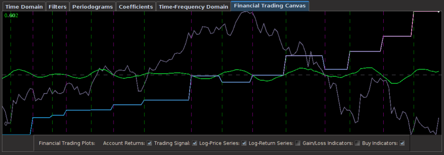
Figure 3: Out-of-sample performance of the signal built without time-shift constraint The out-of-sample period beings where the light cyan line is from Figure 4 below.
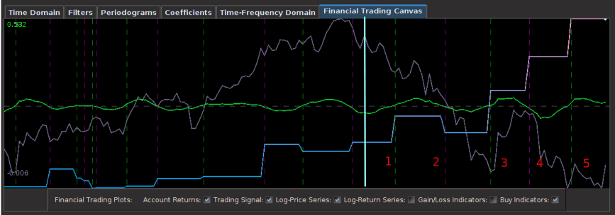
Figure 4: Out-of-sample performance of the signal built with time-shift constraint and optimized for turning point-detection, The out-of-sample period beings where the light cyan is.
Notice how the optimized time-shift constraint in the trading signal in Figure 4 pinpoints to a close perfection where the turning points are (specifically at points 3, 4,and 5). The local minimum turning point was detected exactly at 3, and nearly exact at 4 and 5. The only loss out of the 5 trades occurred at 2, but this was more the fault of the long unexpected fall in the share price of Apple in October. Fortunately we were able to make up for those losses (and then some) at the next trade exactly at the moment a big turning point came (3). Compare this to the non optimized time-shift constrained signal (Figure 3), and how the second and third turning points are a bit too late and too early, respectively. And remember, this performance is all out-of-sample, no adjustments to the filter have been made, nothing adaptive. To see even more clearly how the two signals compare, here are gains and losses of the 5 actual trades performed out-of-sample (all numbers are in percentage according to gains and losses in the trading account governed only by the signal. Positive number is a gain, negative a loss)
Without Time-Shift Optimization With Time-Shift Optimization
Trade 1: 29.1 -> 38.7 = 9.6 14.1 -> 22.3 = 8.2
Trade 2: 38.7 -> 32.0 = -6.7 22.3 -> 17.1 = -5.2
Trade 3: 32.0 -> 40.7 = 8.7 17.1 -> 30.5 = 13.4
Trade 4: 40.7 -> 48.2 = 7.5 30.5 -> 41.2 = 10.7
Trade 5: 48.2 -> 60.2 = 12.0 41.2 -> 53.2 = 12.0
The optimized time-shift signal is clearly better, with an ROI of nearly 40 percent in 3 months of trading. Compare this to roughly 30 percent ROI in the non-constrained signal. I’ll take the optimized time-shift constrained signal any day. I can sleep at night with this type of trading signal. Notice that this trading was applied over a period in which Apple Inc. lost nearly 20 percent of its share price.
Another nice aspect of this trading frequency interval that I used is that trading costs aren’t much of an issue since only 10 transactions (2 transaction each trade) were made in the span of 3 months, even though I did set them to be .01 percent for each transaction nonetheless.
To dig a bit deeper into plausible reasons as to why the optimization of the time-shift constraint matters (if only even just a little bit), let’s take a look at the plots of the coefficients of each respective filter. Figure 5 depicts the filter coefficients with the optimized time-shift constraint, and Figure 6 shows the coefficients without it. Notice how in the filter for the AAPL log-return data (blue-ish tinted line) the filter privileges the latest observation much more, while slowly modifying the others less. In the non optimized time-shift filter, the most recent observation has much less importance, and in fact, privileges a larger lag more. For timely turning point detection, this is (probably) not a good thing. Another interesting observation is that the optimized time-shift filter completely disregards the latest observation in the log-return data of GOOG (purplish-line) in order to determine the turning points. Maybe a “better” financial asset could be used for trading AAPL? Hmmm…. well in any case I’m quite ecstatic with these results so far. I just need to hack my way into writing a better time-shift optimization routine, it’s a bit slow at this point. Until next time, happy extracting. And feel free to contact me with any questions.
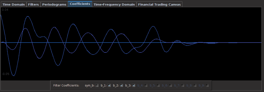
Figure 5: The filter coefficients with time-shift optimization.
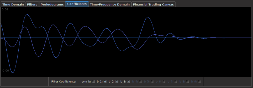
Figure 6: The filter coefficients without the time-shift optimization.
¹ I won’t disclose quite yet how I found these optimal parameters and frequency interval or reveal what they are as I need to keep some sort of competitive advantage as I presently look for consulting opportunities 😉 .


 parameter that controls the phase error in the MDFA optimization. This is done by using the sliding scrollbar marked
  parameter that controls the error in the stop-band between the targeted filter and the computed concurrent filter. The smoothness parameter is found on the Real-Time Filter Design interface in the sliding scrollbar marked
  (see Figure 2) and in the sliding scrollbar marked
  and is found on the Real-Time Filter Design interface (see Figure 2). In theory, as the filter length
  option in the Real-Time Filter Design interface. To go further, one can even set the phase delay to an fixed value other than zero using the
  , which is the reciprocal of the differencing operator in the frequency domain. Since the Financial Trading platform in iMetrica strictly uses log-return financial time series to build trading signals, the use of this weighting function is in a sense a frequency-based “de-differencing” of the differenced data. In many cases, using the differencing weight provides better timeliness properties for the filter and thus the trading signal.
 in the scrollbar to any integer between -10 and 10 and the signal with the set lag applied is automatically computed. For negative lag values