TWS-iMetrica: The Automated Intraday Financial Trading Interface Using Adaptive Multivariate Direct Filtering

Figure 1: The TWS-iMetrica automated financial trading platform. Featuring fast performance optimization, analysis, and trading design features unique to iMetrica for building direct real-time filters to generate automated trading signals for nearly any tradeable financial asset. The system was built using Java, C, and the Interactive Brokers IB API in Java.

Figure 1: The TWS-iMetrica automated financial trading platform. Featuring fast performance optimization, analysis, and trading design features unique to iMetrica for building direct real-time filters to generate automated trading signals for nearly any tradeable financial asset. The system was built using Java, C, and the Interactive Brokers IB API in Java.

Introduction

I realize that I’ve been MIA (missing in action for non-anglophones) the past three months on this blog, but I assure you there has been good reason for my long absence. Not only have I developed a large slew of various optimization, analysis, and statistical tools in iMetrica for constructing high-performance financial trading signals geared towards intraday trading which I will (slowly) be sharing over the next several months (with some of the secret-sauce-recipes kept to myself and my current clients of course), but I have also built, engineered, tested, and finally put into commission on a daily basis the planet’s first automated financial trading platform completely based on the recently developed FT-AMDFA (adaptive multivariate direct filtering approach for financial trading). I introduce to you iMetrica’s little sister, TWS-iMetrica.

Coupled with the original software I developed for hybrid econometrics, time series analysis, signal extraction, and multivariate direct filter engineering called iMetrica, the TWS-iMetrica platform was built in a way to provide an easy to use yet powerful, adaptive, versatile, and automated trading machine for intraday financial trading with a variety of options for building your own day trading strategies using MDFA based on your own financial priorities.  Being written completely in Java and gnu c, the TWS-iMetrica system currently uses the Interactive Brokers (IB) trading workstation (TWS) Java API in order to construct the automated trades, connect to the necessary historical data feeds, and provide a variety of tick data. Thus in order to run, the system will require an activated IB trading account. However, as I discuss in the conclusion of this article, the software was written in a way to be seamlessly adapted to any other brokerage/trading platform API, as long as the API is available in Java or has Java wrappers available.

The steps for setting up and building an intraday financial trading environment using iMetrica + TWS-iMetrica are easy. There are four of them. No technical analysis indicator garbage is used here, no time domain methodologies, or stochastic calculus. TWS-iMetrica is based completely on the frequency domain approach to building robust real-time multivariate filters that are designed to extract signals from tradable financial assets at any fixed observation of frequencies (the most commonly used in my trading experience with FT-AMDFA being 5, 15, 30, or 60 minute intervals). What makes this paradigm of financial trading versatile is the ability to construct trading signals based on your own trading priorities with each filter designed uniquely for a targeted asset to be traded. With that being said, the four main steps using both iMetrica and TWS-iMetrica are as follows:

  1. The first step to building an intraday trading environment is to construct what I call an MDFA portfolio (which I’ll define in a brief moment). This is achieved in the TWS-iMetrica interface that is endowed with a user-friendly portfolio construction panel shown below in Figure 4.
  2. With the desired MDFA portfolio, selected, one then proceeds in connecting TWS-iMetrica to IB by simply pressing the Connect button on the interface in order to download the historical data (see Figure 3).
  3. With the historical data saved, the iMetrica software is then used to upload the saved historical data and build the filters for the given portfolio using the MDFA module in iMetrica (see Figure 2). The filters are constructed using a sequence of proprietary MDFA optimization and analysis tools. Within the iMetrica MDFA module, three different types of filters can be built 1) a trend filter that extracts a fast moving trend 2) a band-pass filter for extracting local cycles, and 3) A multi-bandpass filter that extracts both a slow moving trend and local cycles simultaneously.
  4. Once the filters are constructed and saved in a file (a .cft file), the TWS-iMetrica system is ready to be used for intrady trading using the newly constructed and optimized filters (see Figure 6).
Figure 4: The iMetrica MDFA module for constructing the trading filters. Features dozens of design, analysis, and optimization components to fit the trading priorities of the user and is used in conjunction with the TWS-iMetrica interface.

Figure 2: The iMetrica MDFA module for constructing the trading filters. Features dozens of design, analysis, and optimization components to fit the trading priorities of the user and is used in conjunction with the TWS-iMetrica interface.

In the remaining part of this article, I give an overview of the main features of the TWS-iMetrica software and how easily one can create a high-performing automated trading strategy that fits the needs of the user.

The TWS-iMetrica Interface

The main TWS-iMetrica graphical user interface is composed of several components that allow for constructing a multitude of various MDFA intraday trading strategies, depending on one’s trading priorities. Figure 3 shows the layout of the GUI after first being launched. The first component is the top menu featuring TWS System, some basic TWS connection variables which, in most cases, these variables are left in their default mode, and the Portfolio menu. To access the main menu for setting up the MDFA trading environment, click Setup MDFA Portfolio under the Portfolio menu. Once this is clicked, a panel is displayed (shown in Figure 4) featuring the required a priori parameters for building the MDFA trading environment that should all be filled before MDFA filter construction and trading is to take place. The parameters and their possible values are given below Figure 4.

Figure 3 - The TWS-iMetrica interface when first launched and everything blank.

Figure 3 – The TWS-iMetrica interface when first launched and everything blank.

The Setup MDFA Portfolio panel featuring all the setting necessary to construct the automated trading MDFA environment.

Figure 4 – The Setup MDFA Portfolio panel featuring all the setting necessary to construct the automated trading MDFA environment.

  1. Portfolio – The portfolio is the basis for the MDFA trading platform and consists of two types of assets 1) The target asset from which we construct the trading signal, engineer the trades, and use in building the MDFA filter 2) The explanatory assets that provide the explanatory data for the target asset in the multivariate filter construction. Here, one can select up to four explanatory assets.
  2. Exchange – The exchange on which the assets are traded (according to IB).
  3. Asset Type – If the input portfolio is a selection of Stocks or Futures (Currencies and Options soon to be available).
  4. Expiration – If trading Futures, the expiration date of the contract, given as a six digit number of year then month (e.g. 201306 for June 2013).
  5. Shares/Contracts – The number of shares/contracts to trade (this number can also be changed throughout the trading day through the main panel).
  6. Observation frequency – In the MDFA financial trading method, we consider uniformly sampled observations of market data on which to do the trading (in seconds). The options are 1, 2, 3, 5, 15, 30, and 60 minute data. The default is 5 minutes.
  7. Data – For the intraday observations, determines the nature of data being extracted. Valid values include TRADES, MIDPOINT, BID, ASK, and BID_ASK. The default is MIDPOINT
  8. Historical Data – Selects how many days are used to for downloading the historical data to compute the initial MDFA filters. The historical data will of course come in intervals chosen in the observation frequency.

Once all the values have been set for the MDFA portfolio, click the Set and Build button which will first begin to check if the values entered are valid and if so, create the necessary data sets for TWS-iMetrica to initialize trading. This all must be done while TWS-iMetrica is connected to IB (not set in trading mode however). If the build was successful, the historical data of the desired target financial asset up to the most recent observation in regular market trading hours will be plotted on the graphics canvas. The historical data will be saved to a file named (by default) “lastSeriesData.dat” and the data will be come in columns, where the first column is the date/time of the observation, the second column is the price of the target asset, and remaining columns are log-returns of the target and explanatory data. And that’s it, the system is now setup to be used for financial trading. These values entered in the Setup MDFA Portfolio will never have to be set again (unless changes to the MDFA portfolio are needed of course).

Continuing on to the other controls and features of TWS-iMetrica, once the portfolio has been set, one can proceed to change any of the settings in main trading control panel. All these controls can be used/modified intraday while in automated MDFA trading mode. In the left most side of the panel at the main control panel (Figure 5) of the interface includes a set of options for the following features:

Figure 7 - The main control panel for choosing and/or modifying all the options during intraday trading.

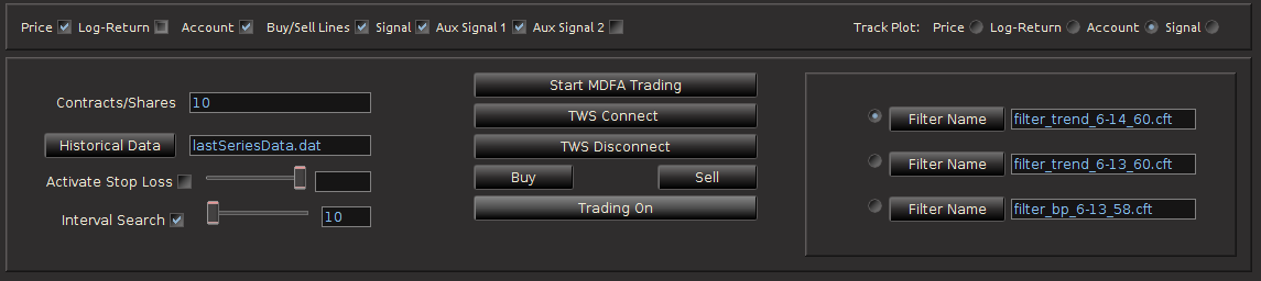
Figure 5 – The main control panel for choosing and/or modifying all the options during intraday trading.

  1. In contracts/shares text field, one enters the amount of share (for stocks) or contracts (for futures)  that one will trade throughout the day. This can be adjusted during the day while the automated trading is activated, however, one must be certain that at the end of the day, the balance between bought and shorted contracts is zero, otherwise, you risk keeping contracts or shares overnight into the next trading day.Typically, this is set at the beginning before automated trading takes place and left alone.
  2. The data input file for loading historical data. The name of this file determines where the historical data associated with the MDFA portfolio constructed will be stored. This historical data will be needed in order to build the MDFA filters. By default this is “lastSeriesData.dat”. Usually this doesn’t need to be modified.
  3. The stop-loss activation and stop-loss slider bar, one can turn on/off the stop-loss and the stop-loss amount. This value determines how/where a stop-loss will be triggered relative to the price being bought/sold at and is completely dependent on the asset being traded.
  4. The interval search that determines how and when the trades will be made when the selected MDFA signal triggers a buy/sell transaction. If turned off, the transaction (a limit order determined by the bid/ask) will be made at the exact time that the buy/sell signal is triggered by the filter. If turned on, the value in the text field next to it gives how often (in seconds) the trade looks for a better price to make the transaction. This search runs until the next observation for the MDFA filter. For example, if 5 minute return data is being used to do the trading, the search looks every seconds for 5 minutes for a better price to make the given transaction. If at the end of the 5 minute period no better price has been found, the transaction is is made at the current ask/bid price. This feature has been shown to be quite useful during sideways or highly volatile markets.

The middle of the main control panel features the main buttons for both connecting to disconnecting from Interactive Brokers, initiating the MDFA automated trading environment, as well as convenient buttons used for instantaneous buy/sell triggers that supplement the automated system. It also features an on/off toggle button for activating the trades given in the MDFA automated trading environment. When checked on, transactions according to the automated MDFA environment will proceed and go through to the IB account. If turned off, the real-time market data feeds and historical data will continue to be read into the TWS-iMetrica system and the signals according to the filters will be automatically computed, but no actual transactions/trades into the IB account will be made.

Finally, on the right hand side of the main control panel features the filter uploading and selection boxes. These are the MDFA filters that are constructed using the MDFA module in iMetrica. One convenient and useful feature of TWS-iMetrica is the ability to utilize up to three direct real-time filters in parallel and to switch at any given moment during market hours between the filters. (Such a feature enhances the adaptability of the trading using MDFA filters. I’ll discuss more about this in further detail shortly).  In order to select up to three filters simultaneously, there is a filter selection panel (shown in bottom right corner of Figure 6 below) displaying three separate file choosers and a radio button corresponding to each filter. Clicking on the filter load button produces a file dialog box from which one selects a filter (a *.cft file produced by iMetrica). Once the filter is loaded properly, on success, the name of the filter is displayed in the text box to the right, and the radio button to the left is enabled. With multiple filters loaded, to select between any of them, simply click on their respective radio button and the corresponding signal will be plotted on the plot canvas (assuming market data has been loaded into the TWS-iMetrica using the market data file upload and/or has been connected to the IB TWS for live market data feeds). This is shown in Figure 6.

Figure 5 - The TWS-iMetrica main trading interface features many control options to design your own automated MDFA trading strategies.

Figure 6 – The TWS-iMetrica main trading interface features many control options to design your own automated MDFA trading strategies.

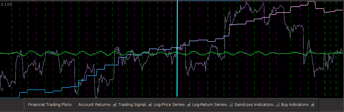
And finally, once the historical data file for the MDFA portfolio has been created, up to three filters have been created for the portfolio and entered in the filter selection boxes, and the system is connected to Interactive Brokers by pressing the Connect button, the market and signal plot panel can then be used for visualizing the different components that one will need for analyzing the market, signal, and performance of the automated trading environment. In the panel just below the plot canvas features and array of checkboxes and radiobuttons. When connected to IB and the Start MDFA Trading has been pressed, all the data and plots are updated in real-time automatically at the specific observation frequency selected in the MDFA Portfolio setup. The currently available plots are as follows:

Figure 8 - The plots for the trading interface. Features price, log-return, account cumulative returns, signal, buy/sell lines, and up to two additional  auxiliary signals.

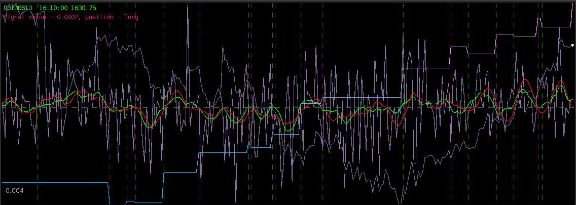
Figure 8 – The plots for the trading interface. Features price, log-return, account cumulative returns, signal, buy/sell lines, and up to two additional auxiliary signals.

  • Price – Plots in real-time the price of the asset being traded, at the specific observation frequency selected for the MDFA portfolio.
  • Log-returns – Plots in real-time the log-returns of the price, which is the data that is being filtered to construct the trading signal.
  • Account – Shows the cumulative returns produced by the currently chosen MDFA filter over the current and historical data period (note that this does not necessary reflect the actual returns made by the strategy in IB, just the theoretical returns over time if this particular filter had been used).
  • Buy/Sell lines – Shows dashed lines where the MDFA trading signal has produced a buy/sell transaction. The green lines are the buy signals (entered a long position) and magenta lines are the sell (entered a short position).
  • Signal – The plot of the signal in real-time. When new data becomes available, the signal is automatically computed and replotted in real-time. This gives one the ability to closely monitory how the current filter is reacting to the incoming data.
  • Aux Signal 1/2 – (If available) Plots of the other available signals produced by the (up to two) other filters constructed and entered in the system. To make either of these auxillary signals the main trading signal simply select the filter associated with the signal using the radio buttons in the filter selection panel.

Along with these plots, to track specific values of any of these plots at anytime, select the desired plot in the Track Plot region of the panel bar. Once selected, specific values and their respective times/dates are displayed in the upper left corner of the plot panel by simply placing the mouse cursor over the plot panel. A small tracking ball will then be moved along the specific plot in accordance with movements by the mouse cursor.

With the graphics panel displaying the performance in real-time of each filter, one can seamlessly switch between a band-pass filter or a timely trend (low-pass) filter according to the changing intraday market conditions. To give an example, suppose at early morning trading hours there is an unusual high amount of volume pushing an uptrend or pulling a downtrend. In such conditions a trend filter is much more appropriate, being able to follow the large-variation in log-returns much better than a band-pass filter can. One can glean from the effects of the trend filter on the morning hours of the market. After automated trading using the trend filter, with the volume diffusing into the noon hour, the band-pass filter can then be applied in order to extract and trade at certain low frequency cycles in the log-return data. Towards the end of the day, with volume continuously picking up, the trend filter can then be selected again in order to track and trade any trending movement automatically.

I am in the process of currently building an automated algorithm to “intelligently” switch between the uploaded filters according to the instantaneous market conditions (with triggering of the switching being set by volume and volatility. Otherwise, for the time being, currently the user must manually switch between different filters, if such switching is at all desired (in most cases, I prefer to leave one filter running all day. Since the process is automated, I prefer to have minimal (if any) interaction with the software during the day while it’s in automated trading mode).

Conclusion

As I mentioned earlier, the main components of the TWS-iMetrica were written in a way to be adaptable to other brokerage/trading APIs. The only major condition is that the API either be available in Java, or at least have (possibly third-party?) wrappers available in Java. That being said, there are only three main types of general calls that are made automated to the connected broker 1) retrieve historical data for any asset(s), at any given time, at most commonly used observation frequencies (e.g. 1 min, 5 min, 10 min, etc.), 2) subscribe to automatic feed of bar/tick data to retrieve latest OHLC and bid/ask data, and finally 3) Place an order (buy/sell) to the broker with different any order conditions (limit, stop-loss, market order, etc.) for any given asset.

If you are interested in having TWS-iMetrica be built for your particular brokerage/trading platform (other than IB of course) and the above conditions for the API are met, I am more than happy to be hired at certain fixed compensation, simply get in contact with me. If you are interested seeing how well the automated system has performed thus far, interested in future collaboration, or becoming a client in order to use the TWS-iMetrica platform, feel free to contact me as well.

Happy extracting!

Advertisement

High-Frequency Financial Trading on Index Futures with MDFA and R: An Example with EURO STOXX50

Figure 1: Out-of-sample performance of the trading signal for the Euro Stoxx50 index futures with expiration March 18th (STXE H3)  during the period of 1-9-2013 and 2-1-2013, using 15 minute log-returns. The black dotted lines indicate a buy/long signal and the blue dotted lines indicate a sell/short (top).

Figure 1: In-sample and Out-of-sample performance (observations 240-457) of the trading signal for the Euro Stoxx50 index futures with expiration March 18th (STXE H3) during the period of 1-9-2013 and 2-1-2013, using 15 minute log-returns. The black dotted lines indicate a buy/long signal and the blue dotted lines indicate a sell/short (top).

In this second tutorial on building high-frequency financial trading signals using the multivariate direct filter approach in R, I focus on the first example of my previous article on signal engineering in high-frequency trading of financial index futures where I consider 15-minute log-returns of the Euro STOXX50 index futures with expiration on March 18th, 2013 (STXE H3).  As I mentioned in the introduction, I added a slightly new step in my approach to constructing the signals for intraday observations as I had been studying the problem of close-to-open variations in the frequency domain. With 15-minute log-return data, I look at the frequency structure related to the close-to-open variation in the price, namely when the price at close of market hours significantly differs from the price at open, an effect I’ve mentioned in my previous two articles dealing with intraday log-return data. I will show (this time in R) how MDFA can take advantage of this variation in price and profit from each one by ‘predicting’ with the extracted signal the jump or drop in the price at the open of the next trading day. Seems to good to be true, right? I demonstrate in this article how it’s possible.

The first step after looking at the log-price and the log-return data of the asset being traded is to construct the periodogram of the in-sample data being traded on.  In this example, I work with the same time frame I did with my previous R tutorial by considering the in-sample portion of my data to be from 1-4-2013 to 1-23-2013, with my out-of-sample data span being from 1-23-2013 to 2-1-2013, which will be used to analyze the true performance of the trading signal. The STXE data and the accompanying explanatory series of the EURO STOXX50 are first loaded into R and then the periodogram is computed as follows.


#load the log-return and log-price SXTE data in-sample
load(paste(path.pgm,"stxe_insamp15min.RData",sep=""))
load(paste(path.pgm,"stxe_priceinsamp15min.RData",sep=""))
#load the log-return and log-price SXTE data out-of-sample
load(paste(path.pgm,"stxe_outsamp15min.RData",sep=""))
load(paste(path.pgm,"stxe_priceoutsamp15min.RData",sep=""))

len_price<-557
out_samp_len<-210
in_samp_len<-347

price_insample<-stxeprice_insamp
price_outsample<-stxeprice_outsamp

#some mdfa definitions
x<-stxe_insamp
len<-length(x[,1])

#my range for the 15-min close-to-open cycle
cutoff<-.32
ub<-.32
lb<-.23

#------------ Compute DFTs ---------------------------
spec_obj<-spec_comp(len,x,0)
weight_func<-spec_obj$weight_func
stxe_periodogram<-abs(spec_obj$weight_func[,1])^2
K<-length(weight_func[,1])-1

#----------- compute Gamma ----------------------------
Gamma<-((0:K)<(K*ub/pi))&((0:K)>(K*lb/pi))

colo<-rainbow(6)
xaxis<-0:K*(pi/(K+1))
plot(xaxis, stxe_periodogram, main="Periodogram of STXE", xlab="Frequency", ylab="Periodogram",
xlim=c(0, 3.14), ylim=c(min(stxe_periodogram), max(stxe_periodogram)),col=colo[1],type="l" )
abline(v=c(ub,lb),col=4,lty=3)

You’ll notice in the periodogram of the in-sample STXE log-returns that I’ve pinpointed a spectral peak between two blue dashed lines. This peak corresponds to an intrinsically important cycle in the 15-minute log-returns of index futures that gives access to predicting the close-to-open variation in the price. As you’ll see, the cycle flows fluidly through the 26 15-minute intervals during each trading day and will cross zero at (usually) one to two points during each trading day to signal whether to go long or go short on the index for the next day. I’ve deduced this optimal frequency range in a prior analysis of this data that I did using my target filter toolkit in iMetrica (see previous article). This frequency range will depend on the frequency of intraday observations, and can also depend on the index (but in my experiments, this range is typically consistent to be between .23 and .32 for most index futures using 15min observations). Thus in the R code above, I’ve defined a frequency cutoff at .32 and upper and lower bandpass cutoffs at .32 and .23, respectively.

Figure 2: Periodogram of the log-return STXE data. The spectral peak is extracted and highlighted between the two red dashed lines.

Figure 2: Periodogram of the log-return STXE data. The spectral peak is extracted and highlighted between the two red dashed lines.

In this first part of the tutorial, I extract this cycle responsible for marking the close-to-open variations and show how well it can perform. As I’ve mentioned in my previous articles on trading signal extraction, I like to begin with the mean-square solution (i.e. no customization or regularization) to the extraction problem to see exactly what kind of parameterization I might need. To produce the plain vanilla mean-square solution, I set all the parameters to 0.0 and then compute the filter by calling the main MDFA function (shown below). The function IMDFA returns an object with the filter coefficients and the in-sample signal. It also plots the concurrent transfer function for both of the filters along with the filter coefficients for increasing lag, shown in Figure 3.

L<-86
lambda_smooth<-0.0
lambda_cross<-0.0
lambda_decay<-c(0.00,0.0)
i1<-F
i2<-F
lambda<-0
expweight<-0
i_mdfa_obj<-IMDFA(L,i1,i2,cutoff,lambda,expweight,lambda_cross,lambda_decay,lambda_smooth,weight_func,Gamma,x)
Figure 3: Concurrent transfer functions for the STXE (red) and explanatory series (cyan) (top). Coefficients for the STXE and explanatory series.

Figure 3: Concurrent transfer functions for the STXE (red) and explanatory series (cyan) (top). Coefficients for the STXE and explanatory series (bottom).

Notice the noise leakage past the stopband in the concurrent filter and the roughness of both sets of filter coefficients (due to overfitting). We would like to smooth both of these out, along with allowing the filter coefficients to decay as the lag increases. This ensures more consistent in-sample and out-of-sample properties of the filter. I first apply some smoothing to the stopband by applying an expweight parameter of 16, and to compensate slightly for this improved smoothness, I improve the timeliness by setting the lambda parameter to 1. After noticing the improvement in the smoothness of filter coefficients, I then proceed with the regularization and conclude with the following parameters.

lambda_smooth<-0.90
lambda_decay<-c(0.08,0.11)
lambda<-1
expweight<-16
Figure 4: Transfer functions and coefficients after smoothing and regularization.

Figure 4: Transfer functions and coefficients after smoothing and regularization.

A vast improvement over the mean-squared solution. Virtually no noise leakage in the stopband passed \omega_1 =.32 
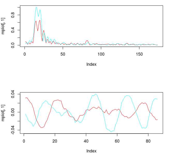
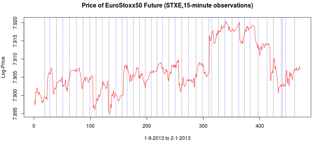
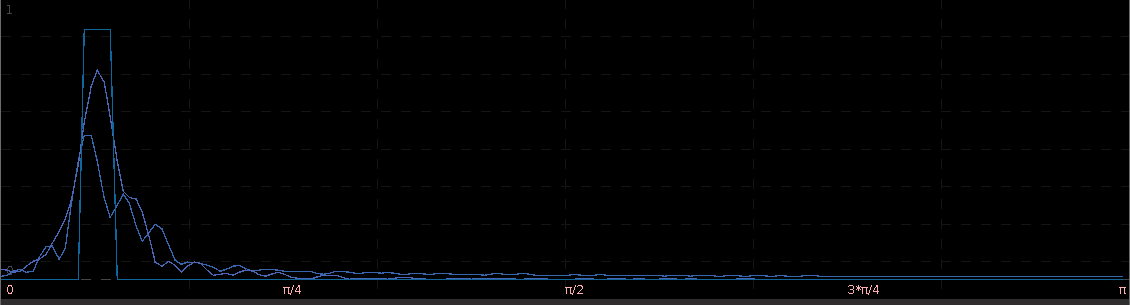
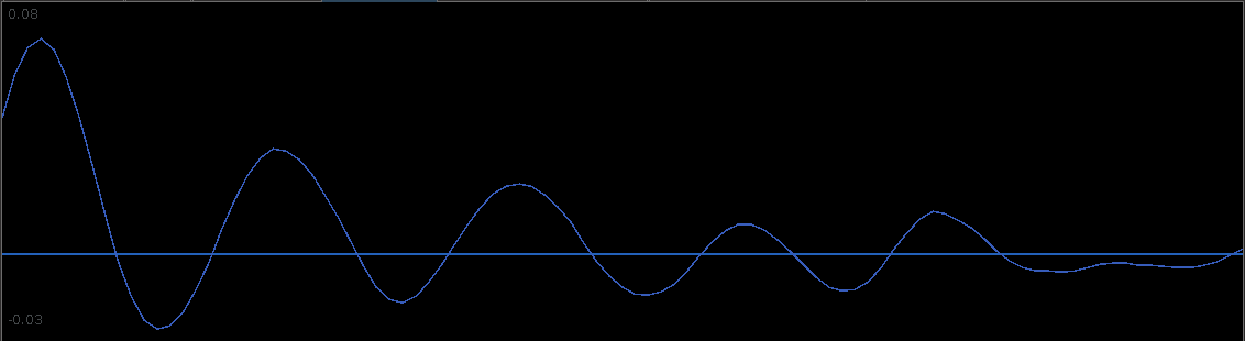
and the coefficients decay beautifully with perfect smoothness achieved. Notice the two transfer functions perfectly picking out the spectral peak that is intrinsic to the close-to-open cycle that I mentioned was between .23 and .32. To verify these filter coefficients achieve the extraction of the close-to-open cycle, I compute the trading signal from the imdfa object and then plot it against the log-returns of STXE. I then compute the trades in-sample using the signal and the log-price of STXE. The R code is below and the plots are shown in Figures 5 and 6.

bn<-i_mdfa_obj$i_mdfa$b
trading_signal<-i_mdfa_obj$xff[,1] + i_mdfa_obj$xff[,2]

plot(x[L:len,1],col=colo[1],type="l")
lines(trading_signal[L:len],col=colo[4])
trade<-trading_logdiff(trading_signal[L:len],price_insample[L:len],0)
Figure : The in-sample signal and the log-returns of SXTE in 15 minute observations from 1-9-2013 to 1-23-2013

Figure 5: The in-sample signal and the log-returns of SXTE in 15 minute observations from 1-9-2013 to 1-23-2013

Figure 5 shows the log-return data and the trading signal extracted from the data. The spikes in the log-return data represent the close-to-open jumps in the STOXX Europe 50 index futures contract, occurring every 27 observations. But notice how regular the signal is, and how consistent this frequency range is found in the log-return data, almost like a perfect sinusoidal wave, with one complete cycle occurring nearly every 27 observations. This signal triggers trades that are shown in Figure 6, where the black dotted lines are buys/long and the blue dotted lines are sells/shorts. The signal is extremely consistent in finding the opportune times to buy and sell at the near optimal peaks, such as at observations 140, 197, and 240. It also ‘predicts’ the jump or fall of the EuroStoxx50 index future for the next trading day by triggering the necessary buy/sell signal, such as at observations 19, 40, 51, 99, 121, 156, and, 250.  The performance of this trading in-sample is shown in Figure 7.

Figure 6: The in-sample trades. Black dotted lines are buy/long and the blue dotted lines are sell/short.

Figure 6: The in-sample trades. Black dotted lines are buy/long and the blue dotted lines are sell/short.

Figure 7: The in-sample performance of the trading signal.

Figure 7: The in-sample performance of the trading signal.

Now for the real litmus test in the performance of this extracted signal, we need to apply the filter out-of-sample to check for consistency in not only performance, but also in trading characteristics. To do this in R, we bind the in-sample and out-of-sample data together and then apply the filter to the out-of-sample set (needing the final L-1 observations from the in-sample portion). The resulting signal in shown in Figure 8.

x_out<-rbind(stxe_insamp,stxe_outsamp)
xff<-matrix(nrow=out_samp_len,ncol=2)

  for(i in 1:out_samp_len)
  {
    xff[i,]<-0
    for(j in 2:3)
    {
      xff[i,j-1]<-xff[i,j-1]+bn[,j-1]%*%x_out[in_samp_len+i:(i-L+1),j]
    }
  }
  trading_signal_outsamp<-xff[,1] + xff[,2]

plot(stxe_outsamp[,1],col=colo[1],type="l")
lines(trading_signal_outsamp,col=colo[4])

The signal and log-return data Notice that the signal performs consistently out-of-sample until right around observation 170 when the log-returns become increasingly volatile. The intrinsic cycle between frequencies .23 and .32 has been slowed down due to this increased volatility and might affect the trading performance.

Figure 9: Out-of-sample signal and log-return data of STXE

Figure 8: Signal produced out-of-sample on 210 observations and log-return data of STXE

The total in-sample plus out-of-sample trading performance is shown in Figure 9 and 10, with the final 210 points being out-of-sample.  The out-of-sample performance is very much akin to the in-sample performance we had, with a very clear systematic trading exposed by ‘predicting’ the next day close-to-open jump or fall in a consistent manner, by triggering the necessary buy/sell signal, such as at observations 310, 363, 383, and 413, with only one loss up until the final day trading.  The higher volatility during the final day of the in-sample period damages the cyclical signal and fails to trade systematically as it had been during the first 420 observations.

Figure 9: The total in-sample plus out-of-sample buys and sells.

Figure 9: The total in-sample plus out-of-sample buys and sells.

Figure 10: Total performance over in-sample and out-of-sample periods.

Figure 10: Total performance over in-sample and out-of-sample periods.

With this kind of performance both in-sample and out-of-sample, and the beautifully consistent yet methodological trading patterns this signal provides, it would seem like attempting to improve upon it would be a pointless task. Why attempt to fix what’s not “broken”. But being the perfectionist that I am, I strive for an even “smarter” filter. If only there was a way to 1) keep the consistent cyclical trading effects as before 2)  ‘predict’ the next day close-to-open jump/fall in the Euro Stoxx50 index future as before, and 3) avoid volatile periods to eliminate erroneous trading, where the signal performed worse. After hours spent in iMetrica, I figured how to do it. This is where advanced trading signal engineering comes into play.

The first step was to include all the lower frequencies below .23, which were not included in my previous trading signal. Due to the low amount of activity in these lower frequencies, this should only provide the effect or a ‘lift’ or a ‘push’ or the signal locally, while still retaining the cyclical component. So after changing my \Gamma to a low-pass filter with cutoff set at \omega = .32, I then computed the filter with the new lowpass design. The transfer functions for the filter coefficients are shown below in Figure 11, with the red colored plot the transfer function for the STXE. Notice that the transfer function for the explanatory series still privileges spectral peak between .23 and .32, with only a slight lift at frequency zero (compare this with the bandpass design in Figure 4, not much has changed).  The problem is that the peak exceeds 1.0 in the passband, and this will amplify the cyclical component extracted from the log-return. It might be okay, trading wise, but not what I’m looking to do.  For the STXE filter, we get slightly more of a lift at frequency zero, however this has been compensated with a decreased cycle extraction between frequencies .23 and .32.  Also, a slight amount of noise has entered in the stopband, another factor we must mollify.


#---- set Gamma to low-pass
cutoff<-.32
Gamma<-((0:K)<(cutoff*K/pi))

#---- compute new filter ----------
i_mdfa_obj<-IMDFA(L,i1,i2,cutoff,lambda,expweight,lambda_cross,lambda_decay,lambda_smooth,weight_func,Gamma,x)
Figure 11: The concurrent transfer functions after changing to lowpass filter.

Figure 11: The concurrent transfer functions after changing to lowpass filter.

To improve the concurrent filter properties for both, I increase the smoothing expweight to 26, which will in turn affect the lambda_smooth, so I decrease it to .70. This gives me a much better transfer function pair, shown in Figure 12.  Notice the peak in the explanatory series transfer function is now much closer to 1.0, exactly what we want.

Figure 11: The concurrent transfer functions after changing to lowpass filter.

Figure 12: The concurrent transfer functions after changing to lowpass filter, increasing expweight to 26, and decreasing lambda_smooth to .70.

I’m still not satisfied with the lift at frequency zero for the STXE series. At roughly .5 at frequency zero, the filter might not provide enough push or pull that I need. The only way to ensure a guaranteed lift in the STXE log-return series is to employ constraints on the filter coefficients so that the transfer function is one at frequency zero. This can be achieved by setting i1 to true in the IMDFA function call, which effectively ensures that the sum of the filter coefficients at \omega = 0 is one. After doing this, I get the following transfer functions and the respective filter coefficients.

#---- Update the regularization parameters
lambda_smooth<-0.68
lambda_cross<-0.0
lambda_decay<-c(0.083,0.11)

#---- update customization parameters
lambda<-0
expweight<-28

#---- set filter constraint -------
i1<-T
weight_constraint[1]<-1
Figure 13: Transfer function and filter coefficients after setting the coefficient constraint i1 to true.

Figure 13: Transfer function and filter coefficients after setting the coefficient constraint i1 to true.

Now this is exactly what I was looking for. Not only does the transfer function for the explanatory series keep the important close-to-open cycle intact, but I have also enforced the lift I need for the STXE series. The coefficients still remain smooth with a nice decaying property at the end.  With the new filter coefficients, I then applied them to the data both in-sample and out-of-sample, yielding the trading signal shown in Figure 14.  It posses exactly the properties that I was seeking. The close-to-open cyclical component is still being extracted (thanks in part to the explanatory series), and is still relatively consistent, although not as much as the pure bandpass design. The feature that I like is the following: When the log-return data diverges away from the cyclical component, with increasing volatility, the STXE filter reacts by pushing the signal down to avoid any erroneous trading. This can be seen in observations 100 through 120 and then at observations 390 through the end of trading. Figure 15 (same as Figure 1 at the top of the article) show the resulting trades and performance produced in-sample and out-of-sample by this signal. This is the art of meticulous signal engineering folks.

Figure 14: In-sample and out-of-sample signal produced from the low-pass with i1 coefficient constraints.

Figure 14: In-sample and out-of-sample signal produced from the low-pass with i1 coefficient constraints.

With only two losses suffered out-of-sample during the roughly 9 days trading, the filter performs much more methodologically than before. Notice during the final two days trading, when volatility picked up, the signal ceases to trade as it is being pushed down. It even continues to ‘predict’ the close-to-open jump/fall correctly, such as at observations 288, 321, and 391. The last trade made was a sell/short sell position, with the signal trending down at the end. The filter is in position to make a huge gain from this timely signaling of a short position at 391, correctly determining a large fall the next trading day, and then waiting out the volatile trading. The gain should be large no matter what happens.

Figure 15: In-sample and out-of-sample performance of the i1 constrained filter design.

Figure 15: In-sample and out-of-sample performance of the i1 constrained filter design.

One thing I mention before concluding is that I made a slight adjustment to my filter design after employing the i1 constraint to get the results shown in Figure 13-15. I’ll leave this as an exercise for the reader to deduce what I have done. Hint: Look at the freezed degrees of freedom before and after applying the i1 constraint. If you still have trouble finding what I’ve done, email me and I’ll give you further hints.

Conclusion

The overall performance of the first filter built, in regards to total return on investment out-of-sample, was superior to the second. However, this superior performance comes only with the assumption that the cycle component defined between frequencies .23 and .32 will continue to be present in future observations of STXE up until the expiration. If volatility increases and this intrinsic cycle ceases to exist in the log-return data, the performance will deteriorate.

For a better more comfortable approach that deals with changing volatile index conditions, I would opt for ensuring that the local-bias is present in the signal, This will effectively push or pull the signal down or up when the intrinsic cycle is weak in the increasing volatility, resulting in a pullback in trading activity.

As before, you can acquire the high-freq data used in this tutorial by requesting it via email.

Happy extracting!

High-Frequency Financial Trading with Multivariate Direct Filtering Part Deux: Index Futures

optimisedstxe

Out-of-sample performance (cash, blue-to-pink line) of an MDFA low-pass filter built using the approach discussed in this article on the STOXX Europe 50 index futures with expiration March 18th (STXEH3) for 200 15-minute interval log-return observations. Only one small loss out-of-sample was recorded from the period of Jan 18th through February 1st, 2013.

Continuing along the trend of my previous installment on strategies and performances of high-frequency trading using multivariate direct filtering, I take on building trading signals for high-frequency index futures, where I will focus on the STOXX Europe 50 Index, S&P 500, and the Australian Stock Exchange Index. As you will discover in this article, these filters that I build using MDFA in iMetrica have yielded some of the best performing trading signals that I have seen using any trading methodology.  My strategy as I’ve been developing throughout my previous articles on MDFA has not changed much, except for one detail that I will discuss throughout and will be a major theme of this article, and that relates to an interesting structure found in index futures series for intraday returns. The structure is related to the close-to-open variation in the price, namely when the price at close of market hours significantly differs from the price at open. an effect I’ve mentioned in my previous two articles dealing with high(er)-frequency (or intraday) log-return data. I will show how MDFA can take advantage of this variation in price and profit from each one by ‘predicting’ with the extracted signal the jump or drop in the price at the open of the next trading day.

The frequency of observations on the index that are to be considered for building trading filters using MDFA is typically only a question of taste and priorities.  The beauty of MDFA lies in not only the versatility and strength in building trading signals for virtually any financial trading priorities, but also in the independence on the underlying observation frequency of the data. In my previous articles, I’ve considered and built high-performing strategies for daily, hourly, and 15 minute log returns, where the focus of the strategy in building the signal began with viewing the periodogram as the main barometer in searching for optimal frequencies on which one should set the low-pass cutoff for the extracting target filter \Gamma function.

Index futures, as in a futures contract on a financial index, as we will see in this article present no new challenges. With the success I had on the 15-minute return observation frequency that I utilized in my previous article in building a signal for the Japanese Yen, I will continue to use the 15 minute intervals for the index futures where I hope to shed some more light on the filter selection process. This includes deducing properties of the intrinsically optimal spectral peaks to trade on. To do this, I present a simple approach I take in these examples by first setting up a bandpass filter over the spectral peak in the periodogram and then study the in-sample and out-of-sample characteristics of this signal, both in performance and consistency. So without further ado, I present my experiments with financial trading on index futures using MDFA, in iMetrica.

STOXX Europe 50 Index (STXE H3, Expiration March 18 2013)

The STOXX Europe 50 Index, Europe’s leading Blue-chip index, provides a representation of sector leaders in Europe. The index covers 50 stocks from 18 European countries and has the highest trading volume of any European index. One of the first things to notice with the 15-minute log-returns of STXE are the frequent large spikes. These spikes will occur every 27 observations at 13:30 (UTC time zone) due to the fact that there are 26 15-minute periods during the trading hours. These spikes represent the close-to-open jumps that the STOXX Europe 50 index has been subjected to and then reflected in the price of the futures contract. With this ‘seasonal’ pattern so obviously present in the log-return data, the frequency effects of this pattern should be clearly visible in the periodogram of the data. The beauty of MDFA (and iMetrica) is that we have the ability to explicitly engineer a trading signal to take advantage of this ‘seasonal’ pattern by building an appropriate extractor \Gamma.

Figure 1: Log-returns of STXE for the 15-min observations from 1-4-2013 to 2-1-2013

Figure 1: Log-returns of STXE for the 15-min observations from 1-4-2013 to 2-1-2013

Regarding the periodogram of the data, Figure 2 depicts the periodograms for the 15 minute log-returns of STXE (red) and the explanatory series (pink) together on the same discretized frequency domain. Notice that in both log-return series, there is a principal spectral peak found between .23 and .32.   The trick is to localize the spectral peak that accounts for the cyclical pattern that is brought about by the close-to-open variation between 20:00 and 13:30 UTC.

Figure 2: The periodograms for the 15 minute log-returns of STXE (red) and the explanatory series (pink).

Figure 2: The periodograms for the 15 minute log-returns of STXE (red) and the explanatory series (pink).

In order to see the effects of the MDFA filter when localizing this spectral peak, I use my target \Gamma builder interface in iMetrica to set the necessary cutoffs for the bandpass filter directly covering both spectral peaks of the log-returns, which are found between .23 and .32. This is shown in Figure 3, where the two dashed red lines show indicate the cutoffs and spectral peak is clearly inside these two cutoffs, with the spectral peak for both series occurring in the vicinity of \pi/12
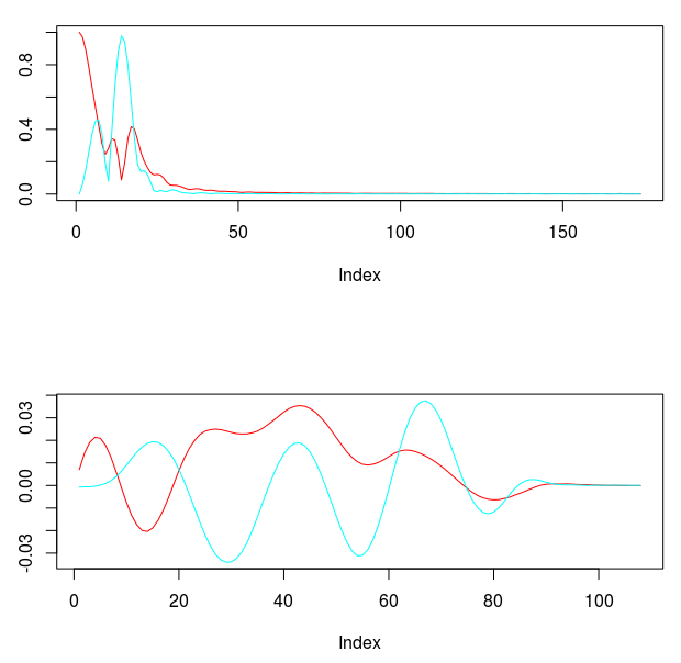
.  Once the bandpass target \Gamma was fixed on this small frequency range, I set the regularization parameters for the filter coefficients to be \lambda_{smooth} = .86,   \lambda_{decay} = .11,  and \lambda_{decay2} = .11.

Figure 3: Choosing the cutoffs for the band pass filter to localize the spectral peak.

Figure 3: Choosing the cutoffs for the band pass filter to localize the spectral peak.

Pinpointing this frequency range that zooms in on the largest spectral peak generates a filter that acts on the intrinsic cycles found in the 15 minute log-returns of the STXE futures index. The resulting trading signal produced by this spectral peak extraction is shown in Figure 4, with the returns (blue to pink line) generated from the trading signal (green) , and the price of the STXE futures index in gray. The cyclical effects in the signal include the close-to-open variations in the data. Notice how the signal predicts the variation of the close-to-open price in the index quite well, seen from the large jumps or falls in price every 27 observations. The performance of this simple design in extracting the spectral peak of STXE yields a 4 percent ROI on 200 observations out-of-sample with only 3 losses out of 20 total trades (85 percent trade success rate), with two of them being accounted for towards the very end of the out-of-sample observations in an uncharacteristic volatile period occurring on January 31st 2013.

Figure : The performance in-sample and out-of-sample of the spectral peak localizing bandpass filter.

Figure 4: The performance in-sample and out-of-sample of the spectral peak localizing bandpass filter.

The two concurrent frequency response (transfer) functions for the two filters acting on the STXE log-return data (purple) and the explanatory series (blue), respectively, are plotted below in Figure 5. Notice the presence of the spectral peaks for both series being accounted for in the vicinity of the frequency \pi/12, with mild damping at the peak. Slow damping of the noise in the higher frequencies is aided by the addition of a smoothing expweight parameter that was set at \alpha = 4.

Figure : The performance in-sample and out-of-sample of the spectral peak localizing bandpass filter.

Figure 5: The concurrent frequency response functions of the localizing spectral peak band-pass filter.

With the ideal characteristics of a trading signal quite present in this simple bandpass filter, namely smooth decaying filter coefficients, in-sample and out-of-sample performance properties identical, and accurate, consistent trading patterns, it would be hard to imagine on improving the trading signal for this European futures index even more. But we can. We simply keep the spectral peak frequencies intact, but also account for the local bias in log-return data by extending the lower cutoff to frequency zero. This will provide improved systematic trading characteristics by not only predicting the close-to-open variation and jumps, but also handling upswings and downswings, and highly volatile periods much better.

In this new design, I created a low-pass filter by keeping the upper cutoff \omega_1 
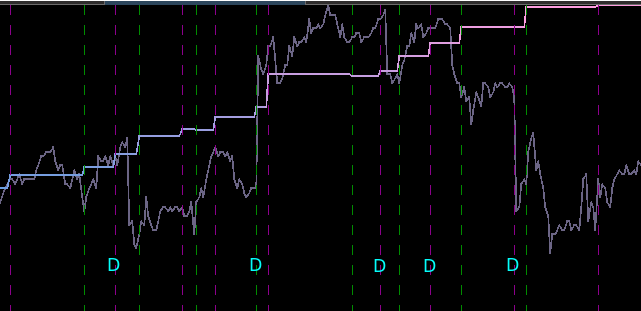
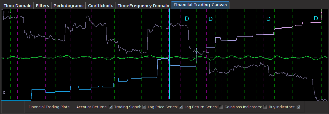
from the band-pass design and setting the lower cutoff to 0. I also increased the smoothing parameter to $\alpha = 32$. In this newly designed filter, we see a vast improvement in the trading structure. As before, the filter was able to deduce the direction of every single close-to-open jump during the 200 out-of-sample observations, but notice that it was also able to become much more flexible in the trading during any upswing/downswing and volatile period. This is seen in more detail in Figure 7, where I added the letter ‘D’ to each of the 5 major buy/sell signals occurring before close.

Figure : Performance of filter both in-sample (left of cyan line) and on 210 observations out-of-sample (right of cyan line).

Figure 6: Performance of filter both in-sample (left of cyan line) and on 210 observations out-of-sample (right of cyan line).

Notice that the signal predicted the jump correctly for each of these major jumps, resulting in large returns. For example, at the first “D” indicator,  the signal indicated sell/short (magenta dashed line) the STXE future index 5 observations before close, namely at 18:45 UTC, before market close at 20:00 UTC. Sure enough, the price of the STXE contract went down during overnight trading hours and opened far below the previous days close, with the filter signaling a buy (green dashed line) 45 minutes into trading. At the mark of the second “D”, we see that on the final observation before market close, the signal produced a buy/long indication, and indeed, the next day the price of the future jumped significantly.

Figure : Zooming in on the out-of-sample performance and showing all the signal responses that predicted the major close-to-open jumps.

Figure 7: Zooming in on the out-of-sample performance and showing all the signal responses that predicted the major close-to-open jumps.

Only two very small losses of less than .08 percent were accounted for.  One advantage of including the frequency zero along with the spectral peak frequency of STXE is that the local bias can help push-up or pull-down the signal resulting in a more ‘patient’ or ‘diligent’ filter that can better handle long upswings/downswings or volatile periods. This is seen in the improvement of the performance towards the end of the 200 observations out-of-sample, where the filter is more patient in signaling a sell/short after the previous buy. Compare this with the end of the performance from the band-pass filter, Figure 4.  With this trading signal out-of-sample, I computed a 5 percent ROI on the 200 observations out-of-sample with only 2 small losses. The trading statistics for the entire in-sample combined with out-of-sample are shown in Figure 8.

Figure 9: The total performance statistics of the STXEH3 trading signal in-sample plus out-of-sample.

Figure 8: The total performance statistics of the STXEH3 trading signal in-sample plus out-of-sample. The max drop indicates -0 due to the fact that there was a truncation to two decimal places. Thus the losses were less than .01.

S&P 500 Futures Index (ES H3, Expiration March 18 2013)

In this experiment trading S&P 500 future contracts (E-mini) on observations of 15 minute intervals from Jan 4th to Feb 1st 2013, I apply the same regimental approach as before.  In looking at the log-returns of ESH3 shown in Figure 10, the effect of close-to-open variation seem to be much less prominent here compared to that on the STXE future index. Because of this, the log-returns seem to be much closer to ‘white noise’ on this index. Let that not perturb our pursuit of a high performing trading signal however. The approach I take for extracting the trading signal, as always, begins with the periodogram.

The log-return data of ES H3 at 15 minute intervals from 1-4-2013 to 2-1-2013.

Figure 10: The log-return data of ES H3 at 15 minute intervals from 1-4-2013 to 2-1-2013.

As the large variations in the close-to-open price are not nearly as prominent, it would make sense that the same spectral peak found before at near \pi/12 is not nearly as prominent either. We can clearly see this in the periodogram plotted below in Figure 11. In fact, the spectral peak at \pi/12 is slightly larger in the explanatory series (pink), thus we should still be able to take advantage of any sort of close-to-open variation that exists in the E-min future index.

Figure 13: Periodograms of ES H3 log-returns (red) and the explanatory series (pink). The red dashed vertical lines are framing the spectral peak between .23 and .32.

Figure 11: Periodograms of ES H3 log-returns (red) and the explanatory series (pink). The red dashed vertical lines are framing the spectral peak between .23 and .32.

With this spectral peak extracted from the series, the resulting trading signal is shown in Figure 12 with the performance of the bandpass signal shown in Figure 13.

Figure 12: The signal built from the extracted spectral peak and the log-return ESH3 data.

Figure 12: The signal built from the extracted spectral peak and the log-return ESH3 data.

One can clearly see that the trading signal performs very well during the consistent cyclical behavior in the ESH3 price, However, when breakdown occurs in this stochastic structure and follows more prominently another frequency, the trading signal dies and no longer trades systematically taking advantage of the intrinsic cycle found near \pi/12. This can be seen in the middle 90 or so observations. The price can be seen to follow more closely a random walk and the trading becomes inconsistent. After this period of 90 or so observations however, just after the beginning of the out-of-sample period, the trajectory of the ESH3 follows back on its consistent course with a \pi/12 cyclical component it had before.

Figure 13: The performance in-sample and out-of-sample of the simple bandpass filter extracting the spectral peak.

Figure 13: The performance in-sample and out-of-sample of the simple bandpass filter extracting the spectral peak.

Now to improve on these results, we include the frequency zero by moving the lower cutoff of the previous band-pass filter to $\latex \omega_0 = 0$.  As I mentioned before, this lifts or pushes down the signal from the local bias and will trade much more systematically. I then lessened the amount of smoothing in the expweight function to \alpha = 24, down from \alpha = 36 as I had on the band-pass filter.  This allows for slightly higher frequencies than \pi/12 to be traded on. I then proceeded to adjust the regularization parameters to obtain a healthy dosage of smoothness and decay in the coefficients. The result of this new low-pass filter design is shown in Figure 14.

Figure 11: Performance out-of-sample (right of cyan line) of the ES H3 filter on 200 15 minute observations.

Figure 14: Performance out-of-sample (right of cyan line) of the ES H3 filter on 200 15 minute observations.

The improvement in the overall systematic trading and performance is clear. Most of the major improvements came from the middle 90 points where the trading became less cyclical. With 6 losses in the band-pass design during this period alone, I was able to turn those losses into two large gains and no losses.  Only one major loss was accounted for during the 200 observation out-of-sample testing of filter from January 18th to February 1st, with an ROI of nearly 4 percent during the 9 trading days. As with the STXE filter in the previous example, I was able to successfully build a filter that correctly predicts close-to-open variations, despite the added difficulty that such variations were much smaller. Both in-sample and out-of-sample, the filter performs consistently, which is exactly what one strives for thanks to regularization.

ASX Futures (YAPH3, Expiration March 18, 2013)

In the final experiment, I build a trading signal for the Australian Stock Exchange futures, during the same period of the previous two experiments. The log-returns show moderately large jumps/drops in price during the entire sample from Jan 4th to Feb 1st, but not quite as large as in the STXE index. We still should be able to take advantage of these close-to-open variations.

YAPH3

Figure 15: The log-returns of the YAPH3 in 15-minute interval observations.

In looking at the periodograms for both the YAPH3 15 minute log-returns (red) and the explanatory series (pink), it is clear that the spectral peaks don’t align like they did in the previous two exampls. In fact, there hardly exists a dominant spectral peak in the explanatory series, whereas the \pi/12 spectral peak in YAPH3 is very prominent. This ultimately might effect the performance of the filter, and consequently the trades. After building the low-pass filter and setting a high smoothing expweight parameter \alpha = 26.5, I then set the regularization parameters to be  \lambda_{smooth} = .85,   \lambda_{decay} = .11,  and \lambda_{decay2} = .11 (same as first example).

Figure : The periodograms for YAPH3 and explanatory series with spectral peak in YAPH3 framed by the red dashed lines.

Figure 16: The periodograms for YAPH3 and explanatory series with spectral peak in YAPH3 framed by the red dashed lines.

The performance of the filter in-sample and out-of-sample is shown in Figure 18. This was one of the more challenging index futures series to work with as I struggled finding an appropriate explanatory series (likely because I was lazy since it was late at night and I was getting tired). Nonetheless, the filter still seems to predict the close-to-open variation on the Australian stock exchange index fairly well. All the major jumps in price are accounted for if you look closely at the trades (green dashed lines are buys/long and magenta lines are sells/shorts) and the corresponding action on the price of the futures contract.   Five losses out-of-sample for a trade success ratio of 72 percent and an ROI out-of-sample on 200 observations of 4.2 percent.  As with all other experiments in building trading signals with MDFA, we check the consistency of the in-sample and out-of-sample performance, and these seem to match up nicely.

Figure : The out-of-sample performance of the low-pass filter on YAPH3.

Figure 18 : The out-of-sample performance of the low-pass filter on YAPH3.

The filter coefficients for the YAPH3 log-difference series is shown in Figure 19. Notice the perfectly smooth undulating yet decaying structure of the coefficients as the lag increases. What a beauty.

Figure 16: Filter coefficients for the YAPH3 series.

Figure 19: Filter coefficients for the YAPH3 series.

Conclusion

Studying the trading performance of spectral peaks by first constructing band-pass filters to extract the signal corresponding to the peak in these index futures enabled me to understand how I can better construct the lowpass filter to yield even better performance. In these examples, I demonstrated that the close-to-open variation in the index futures price can be seen in the periodogram and thus be controlled for in the MDFA trading signal construction. This trading frequency corresponds to roughly \pi/12 in the 15 minute observation data that I had from Jan 4th to Feb 1st. As I witnessed in my empirical studies using iMetrica, this peak is more prominent when the close-to-open variations are larger and more often, promoting a very cyclical structure in the log-return data.  As I look deeper and deeper into studying the effects of extracting spectral peaks in the periodogram of financial data log-returns and the trading performance, I seem to improve on results even more and building the trading signals becomes even easier.

Stay tuned very soon for a tutorial using R (and MDFA) for one of these examples on high-frequency trading on index futures.  If you have any questions or would like to request a certain index future (out of one of the above examples or another) to be dissected in my second and upcoming R tutorial, feel free to shoot me an email.

Happy extracting!

High-Frequency Financial Trading with Multivariate Direct Filtering I: FOREX and Futures

Animation 1: Click to see animation of the Japanese Yen filter in action on 164 hourly out-of-sample observations.

Animation 1: Click to see animation of the Japanese Yen filter in action on 164 hourly out-of-sample observations.

I recently acquired over 300 GBs of financial data that includes tick data for over 7000 financial assets traded on multiple markets for the past 5 years up until February 1st 2013. This USB drive packed with nearly every detail of world financial markets coupled with iMetrica gave me an opportunity to explore at any fashion to my desire the ability of multivariate direct filtering to produce high performance financial trading signals on nearly any high-frequency. Let me begin this article with saying that I am more than ecstatic with the results, as I hope you will too after reading this article.  In this first article in a series of high-frequency trading with MDFA and iMetrica that I plan to write, I provide some initial experiments with building and extracting financial trading signals for high-frequency intraday observations on foreign exchange (FOREX) data, and by high-frequency in the context of this article, I mean higher frequencies than the daily log-returns I’ve been working with in my previous articles. In the first part of this high-frequency series, I begin by exploring hourly, 30 minute, and 15 minute log-returns, and test different strategies, mostly using low-pass and the recently introduced multi-bandpass (MBP) filter to deduce the best approach to tackle the problem of building successful trading signals in higher frequency data.

In my previous articles, I was working uniquely with daily log-return data from different time spans from a year to a year and a half. This enabled the in-sample period of computing the filter coefficients for the signal extraction to include all the most recent annual phases and seasons of markets, from holiday effects, to the transitioning period of August to September that is regularly highly influential on stock market prices and commodities as trading volume increases a significant amount. One immediate question that is raised in migrating to higher-frequency intraday data is what kind of in-sample/out-of-sample time spans should be used to compute the filter in-sample and then for how long do we apply the filter out-of-sample to produce the trades? Another question that is raised with intraday data is how do we account for the close-to-open variation in price? Certainly, after close, the after-hour bids and asks will force a jump into the next trading day. How do we deal with this jump in an optimal manner? As the observation frequency gets higher, say from one hour to 30 minutes, this close-to-open jump/fall should most likely be larger. I will start by saying that, as you will see in the results of this article, with a clever choice of the extractor \Gamma and explanatory series, MDFA can handle these jumps beautifully (both aesthetically and financially). In fact, I would go so far as to say that the MDFA does a superb job in predicting the overnight variation.

One advantage of building trading signals for higher intraday frequencies is that the signals produce trading strategies that are immediately actionable. Namely one can act upon a signal to enter a long or short position immediately when they happen. In building trading signals for the daily log-return, this is not the case since the observations are not actionable points, namely the log difference of today’s ending price with yesterday’s ending price are produced after hours and thus not actionable during open market hours and only actionable the next trading day. Thus trading on intraday observations can lead to better efficiency in trading.

In this first installment in my series on high-frequency financial trading using multivariate direct filtering in iMetrica, I consider building trading signals on hourly returns of foreign exchange currencies. I’ve received a few requests after my recent articles on the Frequency Effect in seeing iMetrica and MDFA in action on the FOREX sector. So to satisfy those curiosities, I give a series of (financially) satisfying and exciting results in combining MDFA and the FOREX. I won’t give all my secretes away into building these signals (as that would of course wipe out my competitive advantage), but I will give some of the parameters and strategies used so any courageously curious reader may try them at home (or the office). In the conclusion, I give a series of even more tricks and hacks.  The results below speak for themselves  So without further ado, let the games begin.

Japanese Yen

Frequency: One hour returns
30 day out-of-sample ROI: 12 percent
Trade success ratio: 92 percent

Yen Filter Parameters: \lambda = 9.2 \alpha = 13.2, \omega_0 = \pi/5
Regularization: smooth = .918, decay = .139, decay2 = .79, cross = 0

In the first experiment, I consider hourly log-returns of a ETF index that mimics the Japanese Yen called FXY. As for one of the explanatory series, I consider the hourly log-returns of the price of GOLD which is traded on NASDAQ. The out-of-sample results of the trading signal built using a low-pass filter and the parameters above are shown in Figure 1.  The in-sample trading signal (left of cyan line) was built using 400 hourly observations of the Yen during US market hours dating back to 1 October 2012. The filter was then applied to the out-of-sample data for 180 hours, roughly 30 trading days up until Friday, 1 February 2013.

Figure 3: Out-of-sample results for the Japanese Yen. The in-sample trading  signal was built using 400 hourly observations of the Yen during US market hours  dating back to November 1st, 2012. The out-of-sample portion passed the cyan line is on 180 hourly observations, about 30 trading days.

Figure 1: Out-of-sample results for the Japanese Yen. The in-sample trading signal was built using 400 hourly observations of the Yen during US market hours dating back to October 1st, 2012. The out-of-sample portion passed the cyan line is on 180 hourly observations, about 30 trading days.

This beauty of this filter is that it yields a trading signal exhibiting all the characteristics that one should strive for in building a robust and successful trading filter.

  1. Consistency: The in-sample portion of the filter performs exactly as it does out-of-sample (after cyan line) in both trade success ratio and systematic trading performance. 
  2. Dropdowns: One small dropdown out-of-sample for a loss of only .8 percent (nearly the cost of the transaction).
  3. Detects the cycles as it should: Although the filter is not able to pinpoint with perfect accuracy every local small upturn during the descent of the Yen against the dollar, it does detect them nonetheless and knows when to sell at their peaks (the magenta lines).
  4. Self-correction: What I love about a robust filter is that it will tend to self-correct itself very quickly to minimize a loss in an erroneous trade. Notice how it did this in the second series of buy-sell transactions during the only loss out-of-sample. The filter detects momentum but quickly sold right before the ensuing downfall. My intuition is that only frequency-based methods such as the MDFA are able to achieve this consistently. This is the sign of a skillfully smart filter.

The coefficients for this Yen filter are shown below. Notice the smoothness of the coefficients from applying the heavy smooth regularization and the strong decay at the very end.  This is exactly the type of smooth/decay combo that one should desire. There is some obvious correlation between the first and second explanatory series in the first 30 lags or so as well. The third explanatory series seems to not provide much support until the middle lags .

Coefficients of the Yen filter. Here we use three different explanatory series to extract  the trading signal shown in Figure 1.

Figure 2: Coefficients of the Yen filter. Here we use three different explanatory series to extract the trading signal.

One of the first things that I always recommend doing when first attempting to build a trading signal is to take a glance at the periodogram. Figure 2 shows the periodogram of the log-return data of the Japanese Yen over 580 hours.  Compare this with the periodogram of the same asset using log-returns of daily data over 580 days, shown in Figure 3.  Notice the much larger prominent spectral peaks at the lower frequencies in the daily log-return data. These prominent spectral peaks renders multibandpass filters much more advantageous and to use as we can take advantage of them by placing a band-pass filter directly over them to extract that particular frequency (see my article on multibandpass filters). However, in the hourly data, we don’t see any obvious spectral peaks to consider, thus I chose a low-pass filter and set the cutoff frequency at $\pi/5$, a standard choice, and good place to begin.

Figure 1: Periodogram of hourly log-returns of the Japanese Yen over 580 hours.

Figure 3: Periodogram of hourly log-returns of the Japanese Yen over 580 hours.

Figure 3: Periodogram of Japanese Yen using 580 daily log-return observations.

Figure 4: Periodogram of Japanese Yen using 580 daily log-return observations. Many more spectral peaks are present in the lower frequencies.

Japanese Yen

Frequency: 15 minute returns
7 day out-of-sample ROI: 5 percent
Trade success ratio: 82 percent

Yen Filter Parameters: \lambda = 3.7 \alpha = 13, \omega_0 = \pi/9
Regularizationsmooth = .90, decay = .11, decay2 = .09, cross = 0

In the next trading experiment, I consider the Japanese Yen again, only this time I look at trading on even high-frequency log-return data than before, namely on 15 minute log-returns of the Yen from the opening bell to market close.  This presents slightly new challenges than before as the close-to-open jumps are much larger than before, but these larger jumps do not necessarily pose problems for the MDFA. In fact, I look to exploit these and take advantage to gain profit by predicting the direction of the jump.  For this higher frequency experiment, I considered 350 15-minute in-sample observations to build and optimize the trading signal, and then applied it over the span of 200 15-minute out-of-sample observations. This produced the results shown in the Figure 5 below. Out of 17 total trades out-of-sample, there were only 3 small losses each less than .5 percent drops and thus 14 gains during the 200 15-minute out-of-sample time period.  The beauty of this filter is its impeccable ability to predict the close-to-open jump in the price of the Yen. Over the nearly 7 day trading span, it was able to correctly deduce whether to buy or short-sell before market close on every single trading day change. In the figure below, the four largest close-to-open variation in Yen price is marked with a “D” and you can clearly see how well the signal was able to correctly deduce a short-sell before market close. This is also consistent with the in-sample performance as well, where you can notice the buys and/or short-sells at the largest close-to-open jumps (notice the large gain in the in-sample period right before the out-of-sample period begins, when the Yen jumped over 1 percent over night.  This performance is most likely aided by the explanatory time series I used for helping predict the close-to-open variation in the price of the Yen. In this example, I only used two explanatory series (the price of Yen, and another closely related to the Yen).

Figure : Out-of-sample performance of the Japanese Yen filter on 15 minute log-return data.

Figure 5: Out-of-sample performance of the Japanese Yen filter on 15 minute log-return data.

We look at the filter transfer functions to see what frequencies they are being privileged in the construction of the filter. Notice that some noise leaks out passed the frequency cutoff at \pi/9, but this is typically normal and a non-issue. I had to balance for both timeliness and smoothness in this filter using both the customization parameters \lambda and \alpha. Not much at frequency 0 is emphasized, with more emphasis stemming from the large spectral peak found right at \pi/9.

Figure : The filter transfer functions.

Figure 6: The filter transfer functions.

British Pound

Frequency: 30 minute returns
14 day out-of-sample ROI: 4 percent
Trade success ratio: 76 percent

British Pound Filter Parameters: \lambda = 5 \alpha = 15, \omega_0 = \pi/9
Regularizationsmooth = .109, decay = .165, decay2 = .19, cross = 0

In this example we consider the frequency of the data to 30 minute returns and attempt to build a robust trading signal for a derivative of the British Pound (BP) on this higher frequency. Instead of using the cash value of the BP, I use 30 minute returns of the BP Futures contract expiring in March (BPH3). Although I don’t have access to tick data from the FOREX, I do have tick data from GLOBEX for the past 5 years.  Thus the futures series won’t be an exact replication of the cash price series of the BP, but it should be quite close due to very low interest rates.

The results of the out-of-sample performance of the BP futures filter are shown in Figure 7. I constructed the filter using an initial in-sample size of 390 30 minute returns dating back to 1 December 2012. After pinpointing a frequency cutoff in the frequency domain for the \Gamma that yielded decent trading results in-sample, I then proceeded to optimize the filter in-sample on smoothness and regularization to achieve similar out-of-sample performance. Applying the resulting filter out-of-sample on 168 30-minute log-return observations of the BP futures series along with 3 explanatory series, I get the results shown below. There were 13 trades made and 10 of them were successful. Notice that the filter does an exquisite job at triggering trades near local optimums associated with the frequencies inside the cutoff of the filter.

Figure 5: The out-of-sample results of the British Pound using 30-minute return data.

Figure 7: The out-of-sample results of the British Pound using 30-minute return data.

In looking at the coefficients of the filter for each series in the extraction, we can clearly see the effects of the regularization: the smoothness of the coefficients the fast decay at the very end. Notice that I never really apply any cross regularization to stress the latitudinal likeliness between the 3 explanatory series as I feel this would detract from the predicting advantages brought by the explanatory series that I used.

Figure 6: The coefficients for the 3 explanatory series of the BP futures,

Figure 8: The coefficients for the 3 explanatory series of the BP futures,

Euro

Frequency: 30 min returns
30 day out-of-sample ROI: 4 percent
Trade success ratio: 71 percent

Euro Filter Parameters: \lambda = 0, \alpha = 6.4, \omega_0 = \pi/9
Regularizationsmooth = .85, decay = .27, decay2 = .12, cross = .001

Continuing with the 30 minute frequency of log-returns, in this example I build a trading signal for the Euro futures contract with expiration on 18 March 2013 (UROH3 on the GLOBEX). My in-sample period, being the same as my previous experiment, is from 1 December 2012 to 4 January 2013 on 30 minute returns using three explanatory time series.  In this example, after inspecting the periodogram, I decided upon a low-pass filter with a frequency cutoff of \pi/9. After optimizing the customization and applying the filter to one month of 30 minute frequency return data out-of-sample (month of January 2013, after cyan line) we see the performance is akin to the performance in-sample, exactly what one strives for. This is due primarily to the heavy regularization of the filter coefficients involved. Only four very small losses of less than .02 percent are suffered during the out-of-sample span that includes 10 successful trades, with the losses only due to the transaction costs. Without transaction costs, there is only one loss suffered at the very beginning of the out-of-sample period.

Figure : Out-of-sample performance on the 30-min log-returns of Euro futures contract UROH3.

Figure 9 : Out-of-sample performance on the 30-min log-returns of Euro futures contract UROH3.

As in the first example using hourly returns, this filter again exhibits the desired characteristics of a robust and high-performing financial trading filter. Notice the out-of-sample performance behaves akin to the in-sample performance, where large upswings and downswings are pinpointed to high-accuracy. In fact, this is where the filter performs best during these periods. No need for taking advantage of a multibandpass filter here, all the profitable trading frequencies are found at less than \pi/9.  Just as with the previous two experiments with the Yen and the British Pound, notice that the filter cleanly predicts the close-to-open variation (jump or drop) in the futures value and buys or sells as needed.  This can be seen from many of the large jumps in the out-of-sample period (after cyan line).

One reason why these trading signals perform so well is due to their approximation power of the symmetric filter. In comparing the trading signal (green) with a high-order approximation of the symmetric filter (gray line) transfer function \Gamma shown in Figure 10, we see that trading signal does an outstanding job at approximating the symmetric filter uniformly. Even at the latest observation (the right most point), the asymmetric filter hones in on the symmetric signal (gray line) with near perfection. Most importantly, the signal crosses zero almost exactly where required.  This is exactly what you want when building a high-performing trading signal.

Figure : Plot of approximation of the real-time trading signal for UROH3 with a high order approximation of the symmetric filter transfer function.

Figure 10: Plot of approximation of the real-time trading signal for UROH3 with a high order approximation of the symmetric filter transfer function.

In looking at the periodogram of the log-return data and the output trading signal differences (colored in blue), we see that the majority of the frequencies were accounted for as expected in comparing the signal with the symmetric signal. Only an inconsequential amount of noise leakage passed the frequency cutoff of \pi/9 is found.  Notice the larger trading frequencies, the more prominent spectral peaks, are located just after \pi/6. These could be taken into account with a smart multibandpass filter in order to manifest even more trades, but I wanted to keep things simple for my first trials with high-frequency foreign exchange data.  I’m quite content with the results that I’ve achieved so far.

Figure : Comparing the periodogram of the signal with the log-return data.

Figure 11: Comparing the periodogram of the signal with the log-return data.

Conclusion

I must admit, at first I was a bit skeptical of the effectiveness that the MDFA would have in building any sort of successful trading signal for FOREX/GLOBEX high frequency data. I always considered the FOREX market rather ‘efficient’ due to the fact that it receives one of the highest trading volumes in the world.  Most strategies that supposedly work well on high-frequency FOREX all seem to use some form of technical analysis or charting (techniques I’m particularly not very fond of), most of which are purely time-domain based. The direct filter approach is a completely different beast, utilizing a transformation into the frequency domain and a ‘bending and warping’ of the metric space for the filter coefficients to extract a signal within the noise that is the log-return data of financial assets.  For the MDFA to be very effective at building timely trading signals, the log-returns of the asset need to diverge from white noise a bit, giving room for pinpointing intrinsically important cycles in the data. However, after weeks of experimenting, I have discovered that building financial trading signals using MDFA and iMetrica on FOREX data is as rewarding as any other.

As my confidence has now been bolstered and amplified even more after my experience with building financial trading signals with MDFA and iMetrica for high-frequency data on foreign exchange log-returns at nearly any frequency, I’d be willing to engage in a friendly competition with anyone out there who is certain that they can build better trading strategies using time domain based methods such as technical analysis or any other statistical arbitrage technique.  I strongly believe these frequency based methods are the way to go, and the new wave in financial trading.  But it takes experience and a good eye for the frequency domain and periodograms to get used to. I haven’t seen many trading benchmarks that utilize other types of strategies, but i’m willing to bet that they are not as consistent as these results using this large of an out-of-sample to in-sample ratio (the ratios in these experiments were between .50 and .80).  If anyone would like to take me up on my offer for a friendly competition (or know anyone that would), feel free to contact me.

After working with a multitude of different financial time series and building many different types of filters, I have come to the point where I can almost eyeball many of the filter parameter choices including the most important ones being the extractor \Gamma along with the regularization parameters, without resorting to time consuming, and many times inconsistent, optimization routines.  Thanks to iMetrica, transitioning from visualizing the periodogram to the transfer functions and to the filter coefficients and back to the time domain to compare with the approximate symmetric filter in order to gauge parameter choices is an easy task, and an imperative one if one wants to build successful trading signals using MDFA.

Here are some overall tips and tricks to build your own high performance trading signals on high-frequency data at home:

  • Pay close attention to the periodogram. This is your best friend in choosing the extractor \Gamma. The best performing signals are not the ones that trade often, but trade on the most important frequencies found in the data. Not all frequencies are created equal. This is true when building either low-pass or multibandpass frequencies. 
  • When tweaking customization, always begin with \alpha, the parameter for smoothness. \lambda for timeliness should be the last resort. In fact, this parameter will most likely be next to useless due to the fact that the log-return of financial data is stationary. You probably won’t ever need it.
  • You don’t need many explanatory series. Like most things in life, quality is superior to quantity. Using the log-return data of the asset you’re trading along with one and maybe two explanatory series that somewhat correlate with the financial asset you’re trading on is sufficient. Anymore than that is ridiculous overkill, probably leading to over-fitting (even the power of regularization at your fingertips won’t help you).

In my next article, I will continue with even more high-frequency trading strategies with the MDFA and iMetrica where I will engage in the sector of Funds and ETFs. If any curious reader would like even more advice/hints/comments on how to build these trading signals on high-frequency data for the FOREX (or the coefficients built in these examples), feel free to get in contact with me via email. I’ll be happy to help.

Happy extracting!

Realizing the Future with iMetrica and HEAVY Models

In this article we steer away from multivariate direct filtering and signal extraction in financial trading and briefly indulge ourselves a bit in the world of analyzing high-frequency financial data, an always hot topic with the ever increasing availability of tick data in computationally convenient formats. Not only has high-frequency intraday data been the basis of higher frequency risk monitoring and forecasting, but it also provides access to building ‘smarter’ volatility prediction models using so-called realized measures of intraday volatility. These realized measures have been shown in numerous studies over the past 5 years or so to provide a solidly more robust indicator of daily volatility.   While daily returns only capture close-to-close volatility, leaving much to be said about the actual volatility of the asset that was witnessed during the day, realized measures of volatility using higher frequency data such as second or minute data provide a much clearer picture of open-to-close variation in trading.

In this article, I briefly describe a new type of volatility model that takes into account these realized measures for volatility movement called  High frEquency bAsed VolatilitY (HEAVY) models developed and pioneered by Shephard and Sheppard 2009. These models take as input both close-to-close daily returns r_t as well as daily realized measures to yield better forecasting dynamics. The models have been shown to be endowed with the ability to not only track momentum in volatility, but also adjust for mean reversion effects as well as adjust quickly to structural breaks in the level of the volatility process.  As the authors (Sheppard and Shephard, 2009) state in their original paper, the focus of these models is on predictive properties, rather than on non-parametric measurement of volatility. Furthermore, HEAVY models are much easier and more robust estimation wise than single source equations (GARCH, Stochastic Volatility) as they bring two sources of volatility information to identify a longer term component of volatility.

The goal of this article is three-fold. Firstly, I briefly review these HEAVY models and give some numerical examples of the model in action using a gnu-c library and Java package called heavy_model that I develped last year for the iMetrica software. The heavy_model package is available for download (either by this link or e-mail me) and features many options that are not available in the MATLAB code provided by Sheppard (bootstrapping methods, Bayesian estimation, track reparameterization, among others). I will then demonstrate the seamless ability to model volatility with these High frEquency bAsed VolatilitY models using iMetrica, where I also provide code for computing realized measures of volatility in Java with the help of an R package called highfrequency (Boudt, Cornelissen, and Payseur 2012).  

HEAVY Model Definition

Let’s denote the daily returns as r_1, r_2, \ldots, r_T, where T is the total amount of days in the sample we are working with. In the HEAVY model, we supplement information to the daily returns by a so-called realized measure of intraday volatility based on higher frequency data, such as second, minute or hourly data. The measures are called daily realized measures and we will denote them as RM_1, RM_2, \ldots, RM_T for the total number of days in the sample.  We can think of these daily realized measures as an average of variance autocorrelations during a single day. They are supposed to provide a better snapshot of the ‘true’ volatility for a specific day t. Although there are numerous ways of computing a realized measure, the easiest is the realized variance computed as RM_t = \sum_j (X_{t+t_{j,t}} - X_{t+t_{j-1,t}})^2 where t_{j,t} are the normalized times of trades on day t. Other methods for providing realized measures includes using Kernel based methods which we will discuss later in this article (see for example http://papers.ssrn.com/sol3/papers.cfm?abstract_id=927483).

Once the realized measures have been computed for T days, the HEAVY model is given by:

Var(r_t | \mathcal{F}_{t-1}^{HF}) = h_t = \omega_1 + \alpha RM_{t-1} + \beta h_{t-1} + \lambda r^2_t

E(RM_t | \mathcal{F}_{t-1}^{HF}) = \mu_t = \omega_2+ \alpha_R RM_{t-1} + \beta_R \mu_{t-1},

where the stability constraints are  \alpha, \omega_1 \geq 0, \beta \in [0,1] and \omega_2, \alpha_R \geq 0 with \lambda + \beta \in [0,1] and \beta_R + \alpha_R \in [0,1]. Here, the \mathcal{F}_{t-1}^{HF} denotes the high-frequency information from the previous day t-1. The first equation models the close-to-close conditional variance and is akin to a GARCH type model, whereas the second equation models the conditional expectation of the open-to-close variation.  

With the formulation above, one can easily see that slight variations to the model are perfectly plausible. For example, one could consider additional lags in either the realized measure RM_t (akin to adding additional moving average parameters) or the conditional mean/variance variable (akin to adding autoregression parameters). One could also leave out the dependence on the squared returns r^2_t by setting \lambda to zero, which is what the original others recommended. A third variation is adding yet another equation to the pack that models a realized measure that takes into account negative and positive momentum to yield possibly better forecasts as it tracks both losses and gains in the model. In this case, one would add the third component by introducing a new equation for a realized semivariance to parametrically model statistical leverage effects, where falls in asset prices are associated with increases in future volatility.  With realized semivariance computed for the T days as RMS_1, \ldots RMS_T, the third equation becomes

E(RMS_t | \mathcal{F}_{t-1}^{HF}) = \phi_t = \omega_3 + \alpha_{RS} RMS_{t-1} + \beta_{RS} \phi_{t-1}

where \alpha_{RS} + \beta_{RS} < 1 and both positive.

HEAVY modeling in C and Java

To incorporate these HEAVY models into iMetrica, I began by writing a gnu-c library for providing a fast and efficient framework for both quasi-likelihood evaluation and a posteriori analysis of the models. The structure of estimating the models follows very closely to the original MATLAB code provided by Sheppard. However, in the c library I’ve added a few more useful tools for forecasting and distribution analysis. The Java code is essentially a wrapper for the c heavy_model library to provide a much cleaner approach to modeling and analyzing the HEAVY data such as the parameters and forecasts.  While there are many ways to declare, implement, and analyze HEAVY models using the c/java toolkit I provide, the most basic steps involved are as follows.

heavyModel heavy = new heavyModel();
heavy.setForecastDimensions(n_forecasts, n_steps);
heavy.setParameterValues(w1, w2, alpha, alpha_R, lambda, beta, beta_R);
heavy.setTrackReparameter(0);
heavy.setData(n_obs, n_series, series);
heavy.estimateHeavyModel();

The first line declares a HEAVY model in java, while the second line sets the number of forecasts samples to compute and how many forecast steps to take. Forecasted values are provided for both the return variable r_t (using a bootstrapping methodology) and the h_t, \mu_t variables. In the next line, the parameter values for the HEAVY model are initialized. These are the initial points that are utilized in the quasi-maximum likelihood optimization routine and can be set to any values that satisfy the model constraints.   Here, w1 = \omega_1, w2 = \omega_2.

The fourth line is completely optional and is used for toggling (0=off, 1=on) a reparameterization of the HEAVY model so the intercepts of both equations in the HEAVY model are explicitly related to the unconditional mean of squared returns r^2 and realized measures RM_t. The reparameterization of the model has the advantage that it eliminates the estimation of \omega_1, \omega_2 and instead uses the unconditional means, leaving two less degrees of freedom in the optimization. See page 12 of the Shephard and Sheppard 2009 paper for a detailed explanation of the reparameterization. After setting the initial values, the data is set for the model by inputting the total number of observation T, the number of series (normally set to 2 and the data in column-wise format (namely a double array of length n_obs x n_series, where the first column is the return data r_t and the second column is the daily realized measure data.  Finally, with the data set and the parameters initialized  we estimate the model in the 6th line. Once the model is finished estimating (should take a few seconds, depending on the number of observations), the heavyModel java object stores the parameter values, forecasts, model residuals, likelihood values, and more. For example, one can print out the estimated model parameters and plot the forecasts of h_t using the following:


heavy.printModelParameters();
heavy.plotForecasts();
Output:
w_1 = 0.063 w_2 = 0.053
beta = 0.855 beta_R = 0.566
alpha = 0.024 alpha_R = 0.375
lambda = 0.087

Figure 1 shows the plot of the filtered h_t, \mu_t values for 300 trading days from June 2011 to June 2012 of AAPL with the final 20 points being the forecasted values. Notice that the multistep ahead forecast shows momentum which is one of the attractive characteristics of the HEAVY models as mentioned in the original paper by Shephard and Sheppard.

Figure 1: Plots of the filtered returns and realized measures with 20 step forecasts for Verizon for 300 trading days.

Figure 1: Plots of the filtered returns and realized measures with 20 step forecasts for Verizon for 300 trading days.

We can also easily plot the estimated joint distribution function F_{\zeta, \eta} by simply using the filtered h_t, \mu_t and computing the devolatilized values \zeta_t = r_t/ \sqrt{h_t}, \eta_t = (RM_t/\mu_t)^{1/2}, leading to the innovations for the model for t = 2,\ldots,T.

Figure 2 below shows the empirical distribution of F_{\zeta, \eta} for 600 days (nearly two years of daily observations from AAPL).  The $\zeta_t$ sequence should be roughly a martingale difference sequences with unit variance and the $\eta_t$ sequence  should have unit conditional means and of course be uncorrelated.  The empirical results validate the theoretical values.

Figure 2: Scatter plot of the empirical distribution of devolatilized values for h and mu.

Figure 2: Scatter plot of the empirical distribution of devolatilized values for h and mu.

In order to compile and run the heavy_model library and the accompanying java wrapper, one must first be sure to meet the requirements for installation. The programs were extensively tested on a 64bit Linux machine running Ubuntu 12.04. The heavy_model library written in c uses the GNU Scientific Library (GSL) for the matrix-vector routines along with a statistical package in gnu-c called apophenia (Klemens, 2012) for the optimization routine. I’ve also included a wrapper for the GSL library called multimin.c which enables using the optimization routines from the GSL library, but were not heavily tested.  The first version (version 00) of the heavy_model library and java wrapper can be downloaded at sourceforge.net/projects/highfrequency.  As a precautionary warning, I must confess that none of the files are heavily commented in any way as this is still a project in progress. Improvements in code, efficiency, and documentation will be continuously coming.

After downloading the .tar.gz package, first ensure that GSL and Apophenia are properly installed and the libraries are correctly installed to the appropriate path for your gnu c compiler. Second, to compile the .c code, copy the makefile.test file to Makefile and then type make. To compile the heavyModel library and utilize the java heavyModel wrapper (recommended), copy makefile.lib to Makefile, then type make. After it constructs the libheavy.so, compile the heavyModel.java file by typing javac heavyModel.java. Note that the java files were complied successfully using the Oracle Java 7 SDK.  If you have any questions about this or any of the c or java files, feel free to contact me. All the files were written by me (except for the optional multimin.c/h files for the optimization) and some of the subroutines (such as the HEAVY model simulation) are based on the MATLAB code by Sheppard. Even though I fully tested and reproduced the results found in other experiments exploring HEAVY models, there still could be bugs in the code. I have not fully tested every aspect (especially the Bayesian estimation components, an ongoing effort) and if anyone would like to add, edit, test, or comment on any of the routines involved in either the c or java code, I’d be more than happy to welcome it.

HEAVY Modeling in iMetrica

The Java wrapper to the gnu-c heavy_model library was installed in the iMetrica software package and can be used for GUI style modeling of high-frequency volatility. The HEAVY modeling environment is a feature of the BayesCronos module in iMetrica that also features other stochastic models for capturing and forecasting volatility such as (E)GARCH, stochastic volatility, mutlivariate stohastic factor modeling, and ARIMA modeling, all using either standard (Q)MLE model estimation or a Bayesian estimation interface (with histograms showing the MCMC results of the parameter chains).

Modeling volatility with HEAVY models is done by first uploading the data into the BayesCronos module (shown in Figure 3) through the use of either the BayesCronos Menu (featured on the top panel) or by using the Data Control Panel (see my previous article on Data Control).

Figure 3: BayesCronos interface in iMetrica for HEAVY modeling.

Figure 3: BayesCronos interface in iMetrica for HEAVY modeling.

In the BayesCronos control panel shown above, we estimate a HEAVY model for the uploaded data (600 observations of r_t, RM_t) that were simulated from a model with omega_1 = 0.05, omega_2 = 0.10, beta = 0.8 beta_R = 0.3, alpha = 0.02, alpha_R = 0.3 (the simulation was done in the Data Control Module).

The model type is selected in the panel under the Model combobox. The number of forecasting steps and forecasting samples (for the r_t variable) are selected in the Forecasting panel. Once those values are set, the model estimates are computed by pressing the “MLE” button in the bottom lower left corner. After the computing is done, all the available plots to analyze the HEAVY model are available by simply clicking the appropriate plotting checkboxes directly below the plotting canvas.   This includes up to 5 forecasts, the original data, the filtered h_t, \mu_t values,  the residuals/empirical distributions of the returns and realized measures, and the pointwise likelihood evaluations for each observation. To see the estimated parameter values, simply click the “Parameter Values” button in the “Model and Parameters” panel and pop-up control panel will appear showing the estimated values for all the parameters.

Realized Measures in iMetrica

Figure : Computing Realized measures in iMetrica using a convenient realized measure control panel.

Figure 4: Computing Realized measures in iMetrica using a convenient realized measure control panel.

Importing and computing realized volatility measures in iMetrica is accomplished by using the control panel shown in Figure 4. With access to high frequency data, one simply types in the ticker symbol in the “Choose Instrument” box, sets the starting and ending date in the standard CCYY-MM-DD format, and then selects the kernel used for assembling the intraday measurements. The Time Scale sets the frequency of the data (seconds, minutes  hours) and the period scrollbar sets the alignment of the data. The Lags combo box determines the bandwidth of the kernel measuring the volatility. Once all the options have been set, clicking on the “Compute Realized Volatility” button will then produce three data sets for the time period given between start date and end data: 1) The daily log-returns of the asset r_1, \ldots, r_T 
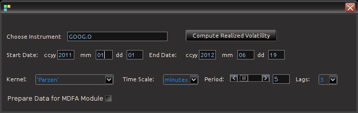
2) The log-price of the asset, and 3) The realized volatility measure RM_1, \ldots, RM_T. Once the Java-R highfrequency routine has finished computing the realized measures, the data sets are automatically available in the Data Control Module of iMetrica. From here, one can annualize the realized measures using the weight adjustments in the Data Control Module (see Figure 5). Once content with the weighting, the data can then be exported to the MDFA module or the BayesCronos module for estimating and forecasting the volatility of GOOG using HEAVY models.

Figure 4: The log-return data (blue) and the (annualized) realized measure data using 5 minute returns (pink).

Figure 5: The log-return data (blue) and the (annualized) realized measure data using 5 minute returns (pink) for Google from 1-1-2011 to 6-19-2012.

The Realized Measure uploading in iMetrica utilizes a fantastic R package for studying and working with high frequency financial data called highfrequency (Boudt, Cornelissen, and Payseur 2012). To handle the analysis of high frequency financial data in java, I began by writing a Java wrapper to the R functions of the highfrequency R package to enable GUI interaction shown above in order to download the data into java and then iMetrica. The java environment uses library called RCaller that opens a live R kernel in the Java runtime environment from which I can call and R routines and directly load the data into Java. The initializing sequence looks like this.


caller.getRCode().addRCode("require (Runiversal)");
caller.getRCode().addRCode("require (FinancialInstrument)");
caller.getRCode().addRCode("require (highfrequency)");
caller.getRCode().addRCode("loadInstruments('/HighFreqDataDirectoryHere/Market/instruments.rda')");
caller.getRCode().addRCode("setSymbolLookup.FI('/HighFreqDataDirectoryHere/Market/sec',use_identifier='X.RIC',extension='RData')");

Here, I’m declaring the R packages that I will be using (first three lines) and then I declare where my HighFrequency financial data symbol lookup directory is on my computer (next two lines). This
then enables me to extract high frequency tick data directly into Java. After loading in the desired intrument ticker symbol names, I then proceed to extract the daily log-returns for the given time frame, and then compute the realized measures of each asset using the rKernelCov function in highfrequency R package. This looks something like

for(i=0;i<n_assets;i++)
{
String mark = instrum[i] + "<-" + instrum[i] + "['T09:30/T16:00',]";

caller.getRCode().addRCode(mark);

String rv = "rv"+i+"<-rKernelCov("+instrum[i]+"$Trade.Price,kernel.type ="+kernels[kern]+", kernel.param="+lags+",kernel.dofadj = FALSE, align.by ="+frequency[freq]+", align.period="+period+", cts=TRUE, makeReturns=TRUE)"

caller.getRCode().addRCode(rv);

caller.getRCode().addRCode("names(rv"+i+")<-'rv"+i+"'");
rvs[i] = "rv_list"+i;

caller.getRCode().addRCode("rv_list"+i+"<-lapply(as.list(rv"+i+"), coredata)");
}

In the first line, I’m looping through all the asset symbols (I create Java strings to load into the RCaller as commands). The second line effectively retrieves the data during market hours only (America/New_York time), then creates a string to call the rKernelCov function in R. I give it all the user defined parameters defined by strings as well. Finally, in the last two lines, I extract the results and put them into an R list from which the java runtime environment will read.

Conclusion

In this article I discussed a recently introduced high frequency based volatility model by Shephard and Sheppard and gave an introduction to three different high-performance tools beyond MATLAB and R that I’ve developed for analyzing these new stochastic models. The heavyModel c/java package that I made available for download gives a workable start for experimenting in a fast and efficient framework the benefit of using high frequency financial data and most notably realized measures of volatility to produce better forecasts. The package will continuously be updated for improvements in both documentation, bug fixes, and overall presentation. Finally, the use of the R package highfrequency embedded in java and then utilized in iMetrica gives a fully GUI experience to stochastic modeling of high frequency financial data that is both conveniently easy to use and fast.

Happy Extracting and Volatilitizing!