Realizing the Future with iMetrica and HEAVY Models

Posted on January 28, 2013 by Christian Dallas Blakely

In this article we steer away from multivariate direct filtering and signal extraction in financial trading and briefly indulge ourselves a bit in the world of analyzing high-frequency financial data, an always hot topic with the ever increasing availability of tick data in computationally convenient formats. Not only has high-frequency intraday data been the basis of higher frequency risk monitoring and forecasting, but it also provides access to building ‘smarter’ volatility prediction models using so-called realized measures of intraday volatility. These realized measures have been shown in numerous studies over the past 5 years or so to provide a solidly more robust indicator of daily volatility. While daily returns only capture close-to-close volatility, leaving much to be said about the actual volatility of the asset that was witnessed during the day, realized measures of volatility using higher frequency data such as second or minute data provide a much clearer picture of open-to-close variation in trading.

In this article, I briefly describe a new type of volatility model that takes into account these realized measures for volatility movement called High frEquency bAsed VolatilitY (HEAVY) models developed and pioneered by Shephard and Sheppard 2009. These models take as input both close-to-close daily returns $r_t$ as well as daily realized measures to yield better forecasting dynamics. The models have been shown to be endowed with the ability to not only track momentum in volatility, but also adjust for mean reversion effects as well as adjust quickly to structural breaks in the level of the volatility process. As the authors (Sheppard and Shephard, 2009) state in their original paper, the focus of these models is on predictive properties, rather than on non-parametric measurement of volatility. Furthermore, HEAVY models are much easier and more robust estimation wise than single source equations (GARCH, Stochastic Volatility) as they bring two sources of volatility information to identify a longer term component of volatility.

The goal of this article is three-fold. Firstly, I briefly review these HEAVY models and give some numerical examples of the model in action using a gnu-c library and Java package called heavy_model that I develped last year for the iMetrica software. The heavy_model package is available for download (either by this link or e-mail me) and features many options that are not available in the MATLAB code provided by Sheppard (bootstrapping methods, Bayesian estimation, track reparameterization, among others). I will then demonstrate the seamless ability to model volatility with these High frEquency bAsed VolatilitY models using iMetrica, where I also provide code for computing realized measures of volatility in Java with the help of an R package called highfrequency (Boudt, Cornelissen, and Payseur 2012).

HEAVY Model Definition

Let’s denote the daily returns as $r_1, r_2, \ldots, r_T$ , where $T$ is the total amount of days in the sample we are working with. In the HEAVY model, we supplement information to the daily returns by a so-called realized measure of intraday volatility based on higher frequency data, such as second, minute or hourly data. The measures are called daily realized measures and we will denote them as $RM_1, RM_2, \ldots, RM_T$ for the total number of days in the sample. We can think of these daily realized measures as an average of variance autocorrelations during a single day. They are supposed to provide a better snapshot of the ‘true’ volatility for a specific day $t$ . Although there are numerous ways of computing a realized measure, the easiest is the realized variance computed as $RM_t = \sum_j (X_{t+t_{j,t}} - X_{t+t_{j-1,t}})^2$ where $t_{j,t}$ are the normalized times of trades on day $t$ . Other methods for providing realized measures includes using Kernel based methods which we will discuss later in this article (see for example http://papers.ssrn.com/sol3/papers.cfm?abstract_id=927483).

Once the realized measures have been computed for $T$ days, the HEAVY model is given by:

$Var(r_t | \mathcal{F}_{t-1}^{HF}) = h_t = \omega_1 + \alpha RM_{t-1} + \beta h_{t-1} + \lambda r^2_t$

$E(RM_t | \mathcal{F}_{t-1}^{HF}) = \mu_t = \omega_2+ \alpha_R RM_{t-1} + \beta_R \mu_{t-1},$

where the stability constraints are $\alpha, \omega_1 \geq 0, \beta \in [0,1]$ and $\omega_2, \alpha_R \geq 0$ with $\lambda + \beta \in [0,1]$ and $\beta_R + \alpha_R \in [0,1]$ . Here, the $\mathcal{F}_{t-1}^{HF}$ denotes the high-frequency information from the previous day $t-1$ . The first equation models the close-to-close conditional variance and is akin to a GARCH type model, whereas the second equation models the conditional expectation of the open-to-close variation.

With the formulation above, one can easily see that slight variations to the model are perfectly plausible. For example, one could consider additional lags in either the realized measure $RM_t$ (akin to adding additional moving average parameters) or the conditional mean/variance variable (akin to adding autoregression parameters). One could also leave out the dependence on the squared returns $r^2_t$ by setting $\lambda$ to zero, which is what the original others recommended. A third variation is adding yet another equation to the pack that models a realized measure that takes into account negative and positive momentum to yield possibly better forecasts as it tracks both losses and gains in the model. In this case, one would add the third component by introducing a new equation for a realized semivariance to parametrically model statistical leverage eﬀects, where falls in asset prices are associated with increases in future volatility. With realized semivariance computed for the $T$ days as $RMS_1, \ldots RMS_T$ , the third equation becomes

$E(RMS_t | \mathcal{F}_{t-1}^{HF}) = \phi_t = \omega_3 + \alpha_{RS} RMS_{t-1} + \beta_{RS} \phi_{t-1}$

where $\alpha_{RS} + \beta_{RS} < 1$ and both positive.

HEAVY modeling in C and Java

To incorporate these HEAVY models into iMetrica, I began by writing a gnu-c library for providing a fast and efficient framework for both quasi-likelihood evaluation and a posteriori analysis of the models. The structure of estimating the models follows very closely to the original MATLAB code provided by Sheppard. However, in the c library I’ve added a few more useful tools for forecasting and distribution analysis. The Java code is essentially a wrapper for the c heavy_model library to provide a much cleaner approach to modeling and analyzing the HEAVY data such as the parameters and forecasts. While there are many ways to declare, implement, and analyze HEAVY models using the c/java toolkit I provide, the most basic steps involved are as follows.

heavyModel heavy = new heavyModel(); heavy.setForecastDimensions(n_forecasts, n_steps); heavy.setParameterValues(w1, w2, alpha, alpha_R, lambda, beta, beta_R); heavy.setTrackReparameter(0); heavy.setData(n_obs, n_series, series); heavy.estimateHeavyModel();

The first line declares a HEAVY model in java, while the second line sets the number of forecasts samples to compute and how many forecast steps to take. Forecasted values are provided for both the return variable $r_t$ (using a bootstrapping methodology) and the $h_t$ , $\mu_t$ variables. In the next line, the parameter values for the HEAVY model are initialized. These are the initial points that are utilized in the quasi-maximum likelihood optimization routine and can be set to any values that satisfy the model constraints. Here, $w1 = \omega_1, w2 = \omega_2$ .

The fourth line is completely optional and is used for toggling (0=off, 1=on) a reparameterization of the HEAVY model so the intercepts of both equations in the HEAVY model are explicitly related to the unconditional mean of squared returns $r^2$ and realized measures $RM_t$ . The reparameterization of the model has the advantage that it eliminates the estimation of $\omega_1, \omega_2$ and instead uses the unconditional means, leaving two less degrees of freedom in the optimization. See page 12 of the Shephard and Sheppard 2009 paper for a detailed explanation of the reparameterization. After setting the initial values, the data is set for the model by inputting the total number of observation $T$ , the number of series (normally set to 2 and the data in column-wise format (namely a double array of length n_obs x n_series, where the first column is the return data $r_t$ and the second column is the daily realized measure data. Finally, with the data set and the parameters initialized we estimate the model in the 6th line. Once the model is finished estimating (should take a few seconds, depending on the number of observations), the heavyModel java object stores the parameter values, forecasts, model residuals, likelihood values, and more. For example, one can print out the estimated model parameters and plot the forecasts of $h_t$ using the following:

heavy.printModelParameters(); heavy.plotForecasts(); Output: w_1 = 0.063 w_2 = 0.053 beta = 0.855 beta_R = 0.566 alpha = 0.024 alpha_R = 0.375 lambda = 0.087

Figure 1 shows the plot of the filtered $h_t, \mu_t$ values for 300 trading days from June 2011 to June 2012 of AAPL with the final 20 points being the forecasted values. Notice that the multistep ahead forecast shows momentum which is one of the attractive characteristics of the HEAVY models as mentioned in the original paper by Shephard and Sheppard.

Figure 1: Plots of the filtered returns and realized measures with 20 step forecasts for Verizon for 300 trading days.

We can also easily plot the estimated joint distribution function $F_{\zeta, \eta}$ by simply using the ﬁltered $h_t, \mu_t$ and computing the devolatilized values $\zeta_t = r_t/ \sqrt{h_t}$ , $\eta_t = (RM_t/\mu_t)^{1/2}$ , leading to the innovations for the model for $t = 2,\ldots,T$ .

Figure 2 below shows the empirical distribution of $F_{\zeta, \eta}$ for 600 days (nearly two years of daily observations from AAPL). The $\zeta_t$ sequence should be roughly a martingale diﬀerence sequences with unit variance and the $\eta_t$ sequence should have unit conditional means and of course be uncorrelated. The empirical results validate the theoretical values.

Figure 2: Scatter plot of the empirical distribution of devolatilized values for h and mu.

In order to compile and run the heavy_model library and the accompanying java wrapper, one must first be sure to meet the requirements for installation. The programs were extensively tested on a 64bit Linux machine running Ubuntu 12.04. The heavy_model library written in c uses the GNU Scientific Library (GSL) for the matrix-vector routines along with a statistical package in gnu-c called apophenia (Klemens, 2012) for the optimization routine. I’ve also included a wrapper for the GSL library called multimin.c which enables using the optimization routines from the GSL library, but were not heavily tested. The first version (version 00) of the heavy_model library and java wrapper can be downloaded at sourceforge.net/projects/highfrequency. As a precautionary warning, I must confess that none of the files are heavily commented in any way as this is still a project in progress. Improvements in code, efficiency, and documentation will be continuously coming.

After downloading the .tar.gz package, first ensure that GSL and Apophenia are properly installed and the libraries are correctly installed to the appropriate path for your gnu c compiler. Second, to compile the .c code, copy the makefile.test file to Makefile and then type make. To compile the heavyModel library and utilize the java heavyModel wrapper (recommended), copy makefile.lib to Makefile, then type make. After it constructs the libheavy.so, compile the heavyModel.java file by typing javac heavyModel.java. Note that the java files were complied successfully using the Oracle Java 7 SDK. If you have any questions about this or any of the c or java files, feel free to contact me. All the files were written by me (except for the optional multimin.c/h files for the optimization) and some of the subroutines (such as the HEAVY model simulation) are based on the MATLAB code by Sheppard. Even though I fully tested and reproduced the results found in other experiments exploring HEAVY models, there still could be bugs in the code. I have not fully tested every aspect (especially the Bayesian estimation components, an ongoing effort) and if anyone would like to add, edit, test, or comment on any of the routines involved in either the c or java code, I’d be more than happy to welcome it.

HEAVY Modeling in iMetrica

The Java wrapper to the gnu-c heavy_model library was installed in the iMetrica software package and can be used for GUI style modeling of high-frequency volatility. The HEAVY modeling environment is a feature of the BayesCronos module in iMetrica that also features other stochastic models for capturing and forecasting volatility such as (E)GARCH, stochastic volatility, mutlivariate stohastic factor modeling, and ARIMA modeling, all using either standard (Q)MLE model estimation or a Bayesian estimation interface (with histograms showing the MCMC results of the parameter chains).

Modeling volatility with HEAVY models is done by first uploading the data into the BayesCronos module (shown in Figure 3) through the use of either the BayesCronos Menu (featured on the top panel) or by using the Data Control Panel (see my previous article on Data Control).

Figure 3: BayesCronos interface in iMetrica for HEAVY modeling.

In the BayesCronos control panel shown above, we estimate a HEAVY model for the uploaded data (600 observations of $r_t, RM_t$ ) that were simulated from a model with omega_1 = 0.05, omega_2 = 0.10, beta = 0.8 beta_R = 0.3, alpha = 0.02, alpha_R = 0.3 (the simulation was done in the Data Control Module).

The model type is selected in the panel under the Model combobox. The number of forecasting steps and forecasting samples (for the $r_t$ variable) are selected in the Forecasting panel. Once those values are set, the model estimates are computed by pressing the “MLE” button in the bottom lower left corner. After the computing is done, all the available plots to analyze the HEAVY model are available by simply clicking the appropriate plotting checkboxes directly below the plotting canvas. This includes up to 5 forecasts, the original data, the filtered $h_t, \mu_t$ values, the residuals/empirical distributions of the returns and realized measures, and the pointwise likelihood evaluations for each observation. To see the estimated parameter values, simply click the “Parameter Values” button in the “Model and Parameters” panel and pop-up control panel will appear showing the estimated values for all the parameters.

Realized Measures in iMetrica

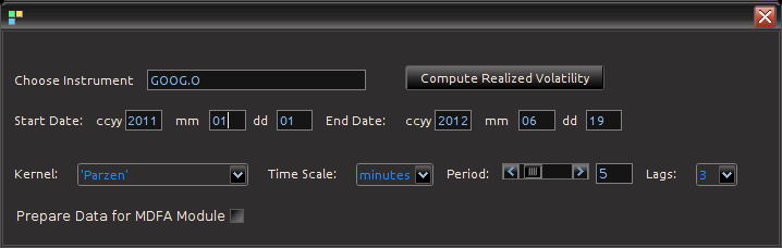
Figure 4: Computing Realized measures in iMetrica using a convenient realized measure control panel.

Importing and computing realized volatility measures in iMetrica is accomplished by using the control panel shown in Figure 4. With access to high frequency data, one simply types in the ticker symbol in the “Choose Instrument” box, sets the starting and ending date in the standard CCYY-MM-DD format, and then selects the kernel used for assembling the intraday measurements. The Time Scale sets the frequency of the data (seconds, minutes hours) and the period scrollbar sets the alignment of the data. The Lags combo box determines the bandwidth of the kernel measuring the volatility. Once all the options have been set, clicking on the “Compute Realized Volatility” button will then produce three data sets for the time period given between start date and end data: 1) The daily log-returns of the asset $r_1, \ldots, r_T$ 2) The log-price of the asset, and 3) The realized volatility measure $RM_1, \ldots, RM_T$ . Once the Java-R highfrequency routine has finished computing the realized measures, the data sets are automatically available in the Data Control Module of iMetrica. From here, one can annualize the realized measures using the weight adjustments in the Data Control Module (see Figure 5). Once content with the weighting, the data can then be exported to the MDFA module or the BayesCronos module for estimating and forecasting the volatility of GOOG using HEAVY models.

Figure 4: The log-return data (blue) and the (annualized) realized measure data using 5 minute returns (pink).

Figure 5: The log-return data (blue) and the (annualized) realized measure data using 5 minute returns (pink) for Google from 1-1-2011 to 6-19-2012.

The Realized Measure uploading in iMetrica utilizes a fantastic R package for studying and working with high frequency financial data called highfrequency (Boudt, Cornelissen, and Payseur 2012). To handle the analysis of high frequency financial data in java, I began by writing a Java wrapper to the R functions of the highfrequency R package to enable GUI interaction shown above in order to download the data into java and then iMetrica. The java environment uses library called RCaller that opens a live R kernel in the Java runtime environment from which I can call and R routines and directly load the data into Java. The initializing sequence looks like this.

caller.getRCode().addRCode("require (Runiversal)"); caller.getRCode().addRCode("require (FinancialInstrument)"); caller.getRCode().addRCode("require (highfrequency)"); caller.getRCode().addRCode("loadInstruments('/HighFreqDataDirectoryHere/Market/instruments.rda')"); caller.getRCode().addRCode("setSymbolLookup.FI('/HighFreqDataDirectoryHere/Market/sec',use_identifier='X.RIC',extension='RData')");
Here, I’m declaring the R packages that I will be using (first three lines) and then I declare where my HighFrequency financial data symbol lookup directory is on my computer (next two lines). This
then enables me to extract high frequency tick data directly into Java. After loading in the desired intrument ticker symbol names, I then proceed to extract the daily log-returns for the given time frame, and then compute the realized measures of each asset using the rKernelCov function in highfrequency R package. This looks something like
for(i=0;i<n_assets;i++) { String mark = instrum[i] + "<-" + instrum[i] + "['T09:30/T16:00',]";

caller.getRCode().addRCode(mark);

String rv = "rv"+i+"<-rKernelCov("+instrum[i]+"$Trade.Price,kernel.type ="+kernels[kern]+", kernel.param="+lags+",kernel.dofadj = FALSE, align.by ="+frequency[freq]+", align.period="+period+", cts=TRUE, makeReturns=TRUE)"

caller.getRCode().addRCode(rv);

caller.getRCode().addRCode("names(rv"+i+")<-'rv"+i+"'"); rvs[i] = "rv_list"+i;

caller.getRCode().addRCode("rv_list"+i+"<-lapply(as.list(rv"+i+"), coredata)"); }

In the first line, I’m looping through all the asset symbols (I create Java strings to load into the RCaller as commands). The second line effectively retrieves the data during market hours only (America/New_York time), then creates a string to call the rKernelCov function in R. I give it all the user defined parameters defined by strings as well. Finally, in the last two lines, I extract the results and put them into an R list from which the java runtime environment will read.

Conclusion

In this article I discussed a recently introduced high frequency based volatility model by Shephard and Sheppard and gave an introduction to three different high-performance tools beyond MATLAB and R that I’ve developed for analyzing these new stochastic models. The heavyModel c/java package that I made available for download gives a workable start for experimenting in a fast and efficient framework the benefit of using high frequency financial data and most notably realized measures of volatility to produce better forecasts. The package will continuously be updated for improvements in both documentation, bug fixes, and overall presentation. Finally, the use of the R package highfrequency embedded in java and then utilized in iMetrica gives a fully GUI experience to stochastic modeling of high frequency financial data that is both conveniently easy to use and fast.

Happy Extracting and Volatilitizing!

iMetrica: Economic and Financial Data Control

Posted on November 14, 2012 by Christian Dallas Blakely

The iMetrica software is endowed with a rich and detailed, yet quite easy-to-use module for uploading, downloading, exporting, editing, combining, transforming, building, simulating, and analyzing time series data. It contains just about anything you’d want to have in an economic or financial time series data control interface while using only simple mouse point-and-click or drag interactions to navigate or download data from the internet. Since the most important aspect of time series analysis is, well, the time series data itself, we created a dedicated data control module to handle the majority of the time series data loading and editing work, before it is exported to any one of the five iMetrica computational modules or financial trading module.

Data Control Interface

We begin this iMetrica blog entry by first giving an overview of the basic components featured in the Data Control module. Figures 1 and 2 show the interface and all the major components labeled. Here, a collection of simulated time series are being plotted together.

Figure 1. The major components of the data control module.

Figure 2. The major components of the data control module, showing the target series editor.

Main plotting canvas. This is where the time series data is plotted. Up to 10 different time series can be loaded into the data control at a time, and all of them can be plotted using the plot control in panel 2. When all the data is plotted together, to highlight a particular series, go to the main Data Control menu in the top left corner and place the mouse on any one the series names, the respective series will then be highlighted.
Plot control panel. The time series that are uploaded into the module can be viewed by toggling their respective check box inside the plot control panel. This is helpful when different time series are scaled different and/or have different means. One can also log-transform the data, rescale the data to have unit standard deviations, or compare data using cross-correlations. Note that the log and rescale check box actions will only apply to the data that is currently being plotted. Furthermore, to plot the cross-correlations, only two time series can be chosen at a time. When one time series is chosen, the auto-correlation plot is drawn. Here, the “Target $X(t)$ indicates a weighted aggregation of the data. To edit this, use the “Target Series” in 3. To delete all of the data stored in the data control module, simply press the “Delete” button. Careful, there’s no going back once deleted.
Simulated and Target Series Panels. The simulated time series data interfaces to simulate a multitude of different time series. Simulating time series can be helpful when wanting to either learn, practice, or explore the different modules and capabilites of iMetrica, learn more about time series analysis, or learn about the dynamics of time series modules. The different types of models include (S)ARIMA models, GARCH models, correlated cycle models, trend models, multivariate factor stochastic volatility models, and HEAVY models. From simulating data and toggling the parameters, one can visualize instantly the effects of the each parameter on the simulated data. The data can then be exported to any of the modules for practicing and honing one’s skills in hybrid modeling, signal extraction, and forecasting. Each model has a “parameter” button (see 4) that controls the dimensions, innovation distributions, or parameter values. When changes are made, the simulated series is recomputed automatically and replotted on their respective plotting canvas (see 4).
Simulated Data Control. Once the parameters have been selected, and a desired simulated series has been achieved to one’s liking, it can be added to the main data control plotting canvas by clicking the “Add” button. The new simulated series is now ready to be exported to any of the modules. One can also change the random seed that controls the “burn-in” of the innovation sequence (random effects that govern the initialization and trajectory of the data). In some of the models, one can “integrate” the data to render stationary data nonstationary.
Parameter Controls. Once the “Parameters” button has been clicked, an additional panel will pop up where controls for all the model’s parameters can be toggled. Once any parameter has been changed using the sliders, scrollbars, or combo boxes, the simulated data is automatically recomputed and plotted, making it a great tool to understand time series model dynamics.
Target Series Construction. The target series is used to construct a univariate time series that is a weighted sum of one or more time series (given by the $X_i(t)$ for $i=1,\ldots,10$ series). In modules that only deal with univariate time series data (the uSimX13, EMD, and State Space Modeling), the constructed target series is the series that gets exported for analysis. For the MDFA module, this is the series that is being filtered for constructing a signal, with the other time series acting as the explanatory time series. In the BayesCronos module, this target series is ignored and only the supporting time series data $X_i(t)$ are used. In these up and down slider controls, one can adjust for the weight associated with that specific series, and the aggregate target series will be automatically recomputed as it is adjusted.
Series Checkboxes. To ignore the series entirely in the computation of the target series, simply click the check box “off” in the associated “computed in target” check box. This will eliminate it from the target sum. In the case one is constructing data for the MDFA module, one has the option of utilizing a series in the target series, but not using it as an explaining time series variable, and vice-versa.

Loading Data from Files

Within this main data control hub, one can import univariate or multivariate time series data from a multitude of file formats, as well as download financial time series data directly from Yahoo! finance or another source such as Reuters for higher-frequency financial data. To load data from a file, simply click on the “Data Input/Export” menu when in the Data Control module and select one of the “Load” data options. The “Load Data” option pop up a “file select” panel and from there, the data file can be selected. The format of the data in this “Load Data” case is simple: a single column of data for each series. If more than one series is present, the data column must be separated by a space. In the “Load CSV” data, this assumes the file is stored in a CSV format. See Figure 3 for the menu options of the Data Control module.

Figure 3. Showing the different options for importing data into the data control module.

Downloading Financial Data

The other option for loading data into the module is through the “Load Market Data” interface. Rather than loading data from a file that is sitting in your directory, you also conveniently have the option to download data directly from the internet or financial time series database, such as Reuters. As a fast and easy way to download financial data into iMetrica, when the “Load Market Data” is selected, a pop-up panel interface will surface that gives access to controlling the download of financial market data. This is shown in Figure 4. The options on this interface are described below.

Figure 4. The “Load Market Data” interface to download market data directly from Yahoo!. Here the daily log-returns and volume of Google (GOOG) and Apple (AAPL) are being downloaded.

Symbols(s) – In this text box, type the market ticker symbol of the desired financial series in all CAPS. Each ticker symbol must be seperated only by one space and nothing else. Up to 10 ticker symbols can be entered.
Start Date – This indicates the year, month, and day from which the financial time series begins. This date must obviously be in the past. If the day falls on a non-traded day such as a weekend or holiday, the nearest date after that date will be chosen. The time series will then be loaded to the most recent date available for that asset.
Hours – This indicates the time period in which the frequency of the data is selected. In most cases, this should simply be set to “US Market Hours”.
Frequency – The frequency of the data. The options are Second, Minute, 3,5,10,15,30-Minute, Hourly, Daily, Weekly, Monthly.
New Data Set – Deletes all the data already stored in the data control module and uploads as new data.
Log Returns – Download the data in log-return format. This is usually the case when using the data to build financial trading strategies using the MDFA module. However, in addition to the log-return data, it will also download the log-transformed raw time series data of the first asset in the Symbols(s) box. This is generally used for gauging financial trading accounts in the financial trading interface of iMetrica. When Financial Trading is turned on in the data control menu this is automatically set on.
Volume Data – In addition to the asset time series data, the volume (of trades) data associated for the given frequency will also be downloaded for each market ticker symbol given in Symbols(s).
Yahoo! Source – The financial data will be downloaded from Yahoo! finance (thus you need an internet connection). If this box is not checked, then the downloader will assume a Reuters financial database (but of course for this you need an account with Reuters).

Once the settings are made in the interface, click “Download Market Data”. If no errors are present in the settings, then all the data should be automatically available in the plot canvas after a few seconds of downloading time. Figure 5 gives the results of the data download from the example in Figure 4. Here, the daily log-returns of Google (GOOG) and Apple (AAPL) along with their daily volumes from 6-4-2011 to today (11-14-2012) have been downloaded into the data control module and ready for use. Notice the scaling of the volume data (final two series) have been adjusted using the simple slider bars in the “Target Series” panel to more-or-less fit the scale of the log-return data.

Figure 5. The daily log-returns of Google (GOOG) and Apple (AAPL) along with their respective volumes loaded into the data control module and plotted on the canvas. The data was uploaded by using the “Load Market Data” interface panel.

If there were errors, then no data will be uploaded to the canvas and you have to try again. Common errors are either no internet connection, the symbols are either incorrect or not in CAPS, or the starting date is bogus. Once the data is available to be plotted, simply click the check boxes associated with each plot. edit, scale, export, analyse, compute, and/or trade away!

More options for downloading data will constantly be added to the iMetrica software. Check back to the blog regularly for more updates and additions as they come. Of course, suggestions are always welcome.

Model comparison with data sweeps

Posted on November 14, 2012 by Christian Dallas Blakely

This slideshow requires JavaScript.

A useful exercise in modeling economic time series is to perform a “sliding window” analysis of the data that computes models in subsets of the data and tests for the robustness of signal extractions, forecasts, and parameter variance relative to a growing subset of the data. For instance, for a time series of length 300, one could estimate a model on a shorter subset of the data, say for the first 200 observations, and then increase the amount of observations, re-estimate, and then see how the model parameter values change as the number of observations or data subset increases. One can also see how the signal extractions and forecasts change with additional data. Ideally, if the model is specified correctly for the data, there should be a very small variance in the estimated parameters as more data is added to the time series. It signifies the stability of the model selection. Normally, such an exercise would be tedious to carry out with X-13ARIMA-SEATS, or any other software such as MATLAB or R as scripts or spec files would have to be written for each individual re-estimation and then re-plotted. In the uSimX13 module of iMetrica however, this task has been rendered an easy one with the addition of a sliding windows tool. In this blog entry, we describe this so-called “sliding windows” process and show just how fast and seamless it is to perform model choice robustness and comparisons in iMetrica.

We begin by describing the sliding span/window tool in the iMetrica-uSimX13 module. Once time series data has been loaded into the uSimX13 module from either the uSimX13 main menu or imported from the Data Control module, the uSimX13 computation engine must first be turned on from the uSimX13 menu. Then to access the sliding windows interface, simply click on the “Sliding Span/Window Activate” check box in the main uSimX13 menu (see Figure 1).

Figure 1. Main drop down menu for the uSimX13 module, showing the “Sliding Span/Window Activate” check box.

Once clicked, the entire plotting canvas will turn to a dark shade of blue, which indicates the windowed region in which model estimation occurs. To control the sliding window, place the mouse cursor along one of the edges of the canvas and slowly glide the mouse with the left-mouse button held down either left or right, depending on which edge of the plot canvas you are on. Moving to the left or right with the left mouse button held down, the windowed area will shrink or expand. The model parameters are estimated instantaneously as the window adjusts and in effect, all the available model statistics, diagnostics, signals, and forecasts are computed as well. For example, as the window expands or shrinks, the trend, seasonally adjusted data, and 24-step ahead forecasts can be plotted and viewed in real-time as the window changes (see Figure 2). One can also slide the window to the left or right by placing the mouse anywhere inside the blue-windowed region, holding down the left mouse button and moving along the time domain. This way, the window length will remain fixed, but the window center will move along different subsets of the data. This can be useful for seeing how model parameters can change within regions of data that exhibit regime changes, namely a sequence in the series that suddenly changes in seasonal or cyclical structure after a certain time observation. The data can now be modeled in both sections before and after the regime change occurs in order to compare the estimated parameter values.

Figure 2. The window sliding across different subsets of the data. The signal extractions, forecast, and model parameters are recomputed automatically as the window changes. Forecast comparisons with the real data as the window span moves is now trivial. Here, the plot in cyan represents the original time series data in-sample and the 24 step forecast out-of-sample, and the light green plot is the time series data adjusted for outliers, as indicated in the model box. One can select the plots using the “series components” plot box. The data in gray represents the time series data not used in the model estimation.

Data Sweep

With the ability to seamlessly capture partitions of the data and model within the given partition using the sliding window, a natural extension of this mouse-on-canvas utility is to employ it somehow in comparing different models of the time series data. We call this method of model comparison time series data sweeping (or simply data sweeping) and it involves selecting an initial window of data from the first observation to the $n$ -th observation where n is some number much less than the total number of observations $latex N$ in the data set (say, one third the amount). The data sweep then computes the sliding window from $n$ as the final observation all the way to $N$ , in increments of one (see Figure 3). At each addition to the length of the window, the forecast is computed for up to 24 steps ahead. Of course, since the true time series data is known in the out-of-sample region of computation, we can compute the forecast error for up to $h \leq 24$ steps ahead and sum up these errors as $n$ increases to $N$ . We can do this data sweep for several models, computing the aggregate forecast errors over time. The idea is that the best model for the data will ideally have the smallest forecast error, and thus comparing this forecast error with several models will identify the model with the best overall forecasting ability.

To access the data sweep, simply go to the main uSimX13 menu, shown in Figure 1, and click “Sweep Time Series Control Panel”. This will bring up the main interface for the data sweep (shown in Figures 4-6). To begin the sweep, first select the model and regressors desired to model the data with inside the model selection panel of the main uSimX13 interface. Then choose at which observation you’d like to carry out the data sweep (starting at observation $n=60$ is the default). Lastly, select how many forecast steps you’d like to use in computing the forecast error (1-24). Once content with the settings, click the “Compute time series sweep” button and watch as the window span increases from $n$ to $N$ , recomputing parameters, signals, and forecasts at each step (see slideshow at top of post). Once the sweep is complete, the parameter statistics, Ljung-Box mean value at two different lags, and the total forecast error is displayed in the control panel. To compare this with another model, save the results of the sweep by clicking “save parameters” in the uSimX13 menu, and then choose another model and recompute (while using the same settings as the previous sweep, of course).

To give an example of this process, we begin by simulating a time series data set of length $N = 300$ from a SARIMA model of dimension $(0,1,2)(0,1,1)_{12}$ , namely a seasonal auto-regressive integrated moving-average process with two non-seasonal moving-average parameters, and one seasonal moving average parameter. The data sweep is performed on the simulated data with a forecast error horizon of length 23 using three different SARIMA models, (a) $(0,1,1)(0,1,1)_{12}$ , (b) $(1,1,0)(0,1,1)_{12}$ , (c) $(0,1,2)(0,1,1)_{12}$ , the true model. See Figures 4-6 below to see the data sweep results and the estimated parameter mean and standard deviation, the average Ljung-Box statistics at lag 12 and 0, and the forecast errors for each model. Notice the forecast error for the true model (c) (figure 6) is the lowest followed by model (b) (figure 6) and then (a) (figure 4), which is exactly what we would want.

Figure 4. Model (a) and the parameter statistics, forecast error, and data sweep controls.

Figure 5. Model (b) and the parameter statistics, forecast error, and data sweep controls.

Figure 6. Model (c) (the true model) and the parameter statistics, forecast error, and data sweep controls.

iMetrica and Hybridometrics: Introduction

Posted on October 24, 2012 by Christian Dallas Blakely

The high-frequency Financial Trading interface of iMetrica. Easily construct in-sample trading strategies with an array of optimizers unique to iMetrica and then employ the strategies out-of-sample to test and fine-tune the trading performance.

This blog serves as an introduction and tutorial to Hybridometrics using iMetrica. Hybridometrics is a term used to express the analysis, modeling, signal extraction, and forecasting of univariate and multivariate financial and economic time series data using a combination of model-based and non-model-based methodologies. Ideal combinations of computational paradigms and methodologies used in hybridometrics include, but are not limited to, traditional stochastic models such as (S)ARIMA models, GARCH models, and multivariate stochastic volatiluty models combined with empirical mode decomposition techniques and the multivariate direct filter approach (MDFA). The goal of hybridometric modeling is to obtain signal extractions and forecasts, for official use or government use, all the way to building high-frequency financial trading strategies, that perform better than using only model or non-model based methods alone. In other words, hybridometrics seeks to extract the advantages of different paradigms combined to outperform traditional approaches to time series modeling. The iMetrica software package offers the most versatile and computationally efficient portal to this newly proposed time series modeling paradigm, all while remaining surprisingly easy to use.

The iMetrica software package is a unique system of econometric and financial trading tools that focuses on speed, user interaction, visualization tools, and point-and-click simplicity in building models for time series data of all types. Written entirely in GNU C and Fortran with a rich interactive interface written in Java, the iMetrica software offers an abundance of econometric tools for signal extraction and forecasting in multivariate time series that are both easily accessible with the click of a mouse button and fast with results computed and plotted instantaneously without the need for creating output data files or calling exterior plotting devices.

One powerful feature that is unique to the iMetrica software is the innate capability of easily combining both model-based and non-model based methodologies for designing data forecasts, signal extraction filters, or high-frequency financial trading strategies. Furthermore, the strategies can be computed and tested both in-sample and out-of-sample using an easy to use built-in data partitioner that effectively partitions the data into an in-sample storage where models and filters are computed and then an out-of-sample storage where new data is applied to the in-sample strategy to test for robustness, over-fitting, and many other desired properties. This gives the user complete liberty in creating a fast and efficient test-bed for implementing signal extractions, forecasting regimes, or financial trading strategies.

The iMetrica software environment includes five interacting time series analysis modules for building hybrid forecasts, signal extractions, and trading strategies.

uSimX13 – A computational environment for univariate seasonal auto-regressive integrated moving-average (SARIMA) modeling and simulation using X-13ARIMA-SEATS. Features an interactive approach to modeling seasonal economic time series with SARIMA models and automatic outlier detection, trading day, and holiday regressor effects. Also includes a suite of model comparison tools using both modern and goodness-of-fit signal extraction diagnostics.
BayesCronos – An interactive time series module for signal extraction and forecasting of multivariate economic and financial time series focusing on Bayesian computation and simulation. This module includes a multitude of models including ARIMA, GARCH, EGARCH, Stochastic Volatility, Multivariate Factor Stochastic Volatility, Dynamic Factor, and Multivariate High-Frequency-Based Volatility (HEAVY), with more models continuously being added. For most of the models featured, one can compute the Bayesian and/or the Quasi-Maximum-Likelihood estimated model fits using either a Metropolis-Hastings Monte Carlo Markov Chain approach (Bayesian) or a QMLE formulation for computing the model parameters estimates. Using a convenient model selection panel interface, complete access to model-type, model parameter dimensions, prior distribution parameters is seamlessly available. In the case of Bayesian estimation, one has complete control over the prior distributions of the model parameters and offers interactive visualization of the Monte Carlo Markov Chain parameter samples. For each model, up to 10 sample 36-steps ahead forecasts can be produced and visualized instantaneously along with other important model features such as model residuals, computed volatility, forecasted volatility, factor models, and more. The results can then be easily exported to other modules in iMetrica for additional filtering and/or modeling.
MDFA – An interactive interface to the most comprehensive multivariate real-time direct filter analysis and computation environment in the world. Build real-time filters using both I-MDFA and Zero-Pole Combination (ZPC) filter constructions. The module includes interactive access to timeliness, smoothing, and accuracy controls for filter customization along with parameters for filter regularization to control overfitting. More advanced features include an interface for building adaptive filters, and many controls for filter optimization, customization, data forecasting, and target filter construction.
State Space Modeling – A module for building observed component ARIMA and regression models for univariate economic time series. Similar to the uSimX13 module, the State Space Modeling environment focuses on modeling and forecasting economic time series data, but with much more generality than SARIMA models. An aggregation of observed stochastic components in the form of ARIMA models are stipulated for the time series data (for example trend + seasonal + irregular) and then regression components to model outliers, holiday, and trading day effects are added to the stochastic components giving ultimate flexibility in model building. The module uses regCMPNT, a suite of Fortran code written at the US Census Bureau, for the maximum likelihood and Kalman filter computational routines.
EMD – The EMD module offers a time-frequency decomposition environment for the time-frequency analysis of time series data. The module offers both the original empirical mode decomposition technique of Huan et al. using cubic splines, along with an adaptive approach using reproducing kernels and direct-filtering. This empirical decomposition technique decomposes nonlinear and nonstationary time series into amplitude modulated and frequency modulated (AM-FM) components and then computes the intrinsic phase and instantaneous frequency components from the FM components. All plots of the components as well as the time-frequency heat maps are generated instantaneously.

Along with these modules, there is also a data control module that handles all aspects of time series data input and export. Within this main data control hub, one can import multivariate time series data from a multitude of file formats, as well as download financial time series data directly from Yahoo! finance or another source such as Reuters for higher-frequency financial data. Once the data is loaded, the data can be normalized, scaled, demeaned, and/or log-transformed with a simple slider and button controls, with the effects being plotted on the graphic canvas instantaneously.

Another great feature of the iMetrica software is the ability to learn more about time series modeling through the using of data simulators. The data control module includes an array of data simulating panels for simulating data from a multitude of both univariate and multivariate time series models. With access to control the number of observations, the random seed for the innovation process, the innovation process distribution, and the model parameters, simulated data can be constructed for any type of economic or financial time time series imaginable. The different types of models include (S)ARIMA models, GARCH models, correlated cycle models, trend models, multivariate factor stochastic volatility models, and HEAVY models. From simulating data and toggling the parameters, one can visualize instantly the effects of the each parameter on the simulated data. The data can then be exported to any of the modules for practicing and honing one’s skills in hybrid modeling, signal extraction, and forecasting.

Keep visiting this blog frequently for continuous updates, tutorials, and proposals in the field of econometrics, signal extraction, forecasting, and high-frequency financial trading. using hybridometrics and iMetrica.

Hybrid Signal Extraction, Machine Learning, and Algorithmic Financial Trading

Combining Computational Methodologies for Real-Time Learning and Signal Extraction

Tag Archives: econometrics