In this article we steer away from multivariate direct filtering and signal extraction in financial trading and briefly indulge ourselves a bit in the world of analyzing high-frequency financial data, an always hot topic with the ever increasing availability of tick data in computationally convenient formats. Not only has high-frequency intraday data been the basis of higher frequency risk monitoring and forecasting, but it also provides access to building ‘smarter’ volatility prediction models using so-called realized measures of intraday volatility. These realized measures have been shown in numerous studies over the past 5 years or so to provide a solidly more robust indicator of daily volatility. While daily returns only capture close-to-close volatility, leaving much to be said about the actual volatility of the asset that was witnessed during the day, realized measures of volatility using higher frequency data such as second or minute data provide a much clearer picture of open-to-close variation in trading.
In this article, I briefly describe a new type of volatility model that takes into account these realized measures for volatility movement called High frEquency bAsed VolatilitY (HEAVY) models developed and pioneered by Shephard and Sheppard 2009. These models take as input both close-to-close daily returns  as well as daily realized measures to yield better forecasting dynamics. The models have been shown to be endowed with the ability to not only track momentum in volatility, but also adjust for mean reversion effects as well as adjust quickly to structural breaks in the level of the volatility process. As the authors (Sheppard and Shephard, 2009) state in their original paper, the focus of these models is on predictive properties, rather than on non-parametric measurement of volatility. Furthermore, HEAVY models are much easier and more robust estimation wise than single source equations (GARCH, Stochastic Volatility) as they bring two sources of volatility information to identify a longer term component of volatility.
The goal of this article is three-fold. Firstly, I briefly review these HEAVY models and give some numerical examples of the model in action using a gnu-c library and Java package called heavy_model that I develped last year for the iMetrica software. The heavy_model package is available for download (either by this link or e-mail me) and features many options that are not available in the MATLAB code provided by Sheppard (bootstrapping methods, Bayesian estimation, track reparameterization, among others). I will then demonstrate the seamless ability to model volatility with these High frEquency bAsed VolatilitY models using iMetrica, where I also provide code for computing realized measures of volatility in Java with the help of an R package called highfrequency (Boudt, Cornelissen, and Payseur 2012).
HEAVY Model Definition
Let’s denote the daily returns as  , where
  is the total amount of days in the sample we are working with. In the HEAVY model, we supplement information to the daily returns by a so-called realized measure of intraday volatility based on higher frequency data, such as second, minute or hourly data. The measures are called daily realized measures and we will denote them as
  for the total number of days in the sample. We can think of these daily realized measures as an average of variance autocorrelations during a single day. They are supposed to provide a better snapshot of the ‘true’ volatility for a specific day
  . Although there are numerous ways of computing a realized measure, the easiest is the realized variance computed as
  where
where  are the normalized times of trades on day . Other methods for providing realized measures includes using Kernel based methods which we will discuss later in this article (see for example http://papers.ssrn.com/sol3/papers.cfm?abstract_id=927483).
Once the realized measures have been computed for days, the HEAVY model is given by:


where the stability constraints are ![\alpha, \omega_1 \geq 0, \beta \in [0,1]](https://s0.wp.com/latex.php?latex=%5Calpha%2C+%5Comega_1+%5Cgeq+0%2C+%5Cbeta+%5Cin+%5B0%2C1%5D&bg=ffffff&fg=323232&s=0&c=20201002) and
and  with
with ![\lambda + \beta \in [0,1]](https://s0.wp.com/latex.php?latex=%5Clambda+%2B+%5Cbeta+%5Cin+%5B0%2C1%5D&bg=ffffff&fg=323232&s=0&c=20201002) and
and ![\beta_R + \alpha_R \in [0,1]](https://s0.wp.com/latex.php?latex=%5Cbeta_R+%2B+%5Calpha_R+%5Cin+%5B0%2C1%5D&bg=ffffff&fg=323232&s=0&c=20201002) . Here, the
. Here, the  denotes the high-frequency information from the previous day
  . The first equation models the close-to-close conditional variance and is akin to a GARCH type model, whereas the second equation models the conditional expectation of the open-to-close variation.
With the formulation above, one can easily see that slight variations to the model are perfectly plausible. For example, one could consider additional lags in either the realized measure  (akin to adding additional moving average parameters) or the conditional mean/variance variable (akin to adding autoregression parameters). One could also leave out the dependence on the squared returns
  by setting
  to zero, which is what the original others recommended. A third variation is adding yet another equation to the pack that models a realized measure that takes into account negative and positive momentum to yield possibly better forecasts as it tracks both losses and gains in the model. In this case, one would add the third component by introducing a new equation for a realized semivariance to parametrically model statistical leverage effects, where falls in asset prices are associated with increases in future volatility. With realized semivariance computed for the days as
  , the third equation becomes

where  and both positive.
HEAVY modeling in C and Java
To incorporate these HEAVY models into iMetrica, I began by writing a gnu-c library for providing a fast and efficient framework for both quasi-likelihood evaluation and a posteriori analysis of the models. The structure of estimating the models follows very closely to the original MATLAB code provided by Sheppard. However, in the c library I’ve added a few more useful tools for forecasting and distribution analysis. The Java code is essentially a wrapper for the c heavy_model library to provide a much cleaner approach to modeling and analyzing the HEAVY data such as the parameters and forecasts. While there are many ways to declare, implement, and analyze HEAVY models using the c/java toolkit I provide, the most basic steps involved are as follows.
 heavyModel heavy = new heavyModel();

heavy.setForecastDimensions(n_forecasts, n_steps);

heavy.setParameterValues(w1, w2, alpha, alpha_R, lambda, beta, beta_R);

heavy.setTrackReparameter(0);

heavy.setData(n_obs, n_series, series);

heavy.estimateHeavyModel();
The first line declares a HEAVY model in java, while the second line sets the number of forecasts samples to compute and how many forecast steps to take. Forecasted values are provided for both the return variable (using a bootstrapping methodology) and the  ,
,  variables. In the next line, the parameter values for the HEAVY model are initialized. These are the initial points that are utilized in the quasi-maximum likelihood optimization routine and can be set to any values that satisfy the model constraints. Here,
  .
.
The fourth line is completely optional and is used for toggling (0=off, 1=on) a reparameterization of the HEAVY model so the intercepts of both equations in the HEAVY model are explicitly related to the unconditional mean of squared returns  and realized measures . The reparameterization of the model has the advantage that it eliminates the estimation of
  and instead uses the unconditional means, leaving two less degrees of freedom in the optimization. See page 12 of the Shephard and Sheppard 2009 paper for a detailed explanation of the reparameterization. After setting the initial values, the data is set for the model by inputting the total number of observation , the number of series (normally set to 2 and the data in column-wise format (namely a double array of length n_obs x n_series, where the first column is the return data and the second column is the daily realized measure data. Finally, with the data set and the parameters initialized we estimate the model in the 6th line. Once the model is finished estimating (should take a few seconds, depending on the number of observations), the heavyModel java object stores the parameter values, forecasts, model residuals, likelihood values, and more. For example, one can print out the estimated model parameters and plot the forecasts of using the following:
heavy.printModelParameters();

heavy.plotForecasts();

Output:

w_1 = 0.063 w_2 = 0.053

beta = 0.855 beta_R = 0.566

alpha = 0.024 alpha_R = 0.375

lambda = 0.087
Figure 1 shows the plot of the filtered  values for 300 trading days from June 2011 to June 2012 of AAPL with the final 20 points being the forecasted values. Notice that the multistep ahead forecast shows momentum which is one of the attractive characteristics of the HEAVY models as mentioned in the original paper by Shephard and Sheppard.
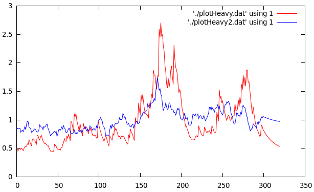
Figure 1: Plots of the filtered returns and realized measures with 20 step forecasts for Verizon for 300 trading days.
We can also easily plot the estimated joint distribution function  by simply using the filtered and computing the devolatilized values
  ,
,  , leading to the innovations for the model for
  .
.
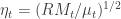
Figure 2 below shows the empirical distribution of for 600 days (nearly two years of daily observations from AAPL). The $\zeta_t$ sequence should be roughly a martingale difference sequences with unit variance and the $\eta_t$ sequence should have unit conditional means and of course be uncorrelated. The empirical results validate the theoretical values.
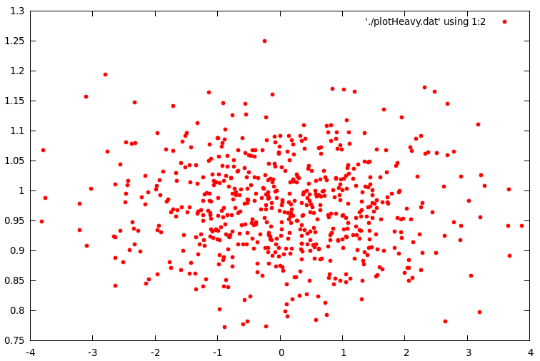
Figure 2: Scatter plot of the empirical distribution of devolatilized values for h and mu.
In order to compile and run the heavy_model library and the accompanying java wrapper, one must first be sure to meet the requirements for installation. The programs were extensively tested on a 64bit Linux machine running Ubuntu 12.04. The heavy_model library written in c uses the GNU Scientific Library (GSL) for the matrix-vector routines along with a statistical package in gnu-c called apophenia (Klemens, 2012) for the optimization routine. I’ve also included a wrapper for the GSL library called multimin.c which enables using the optimization routines from the GSL library, but were not heavily tested. The first version (version 00) of the heavy_model library and java wrapper can be downloaded at sourceforge.net/projects/highfrequency. As a precautionary warning, I must confess that none of the files are heavily commented in any way as this is still a project in progress. Improvements in code, efficiency, and documentation will be continuously coming.
After downloading the .tar.gz package, first ensure that GSL and Apophenia are properly installed and the libraries are correctly installed to the appropriate path for your gnu c compiler. Second, to compile the .c code, copy the makefile.test file to Makefile and then type make. To compile the heavyModel library and utilize the java heavyModel wrapper (recommended), copy makefile.lib to Makefile, then type make. After it constructs the libheavy.so, compile the heavyModel.java file by typing javac heavyModel.java. Note that the java files were complied successfully using the Oracle Java 7 SDK. If you have any questions about this or any of the c or java files, feel free to contact me. All the files were written by me (except for the optional multimin.c/h files for the optimization) and some of the subroutines (such as the HEAVY model simulation) are based on the MATLAB code by Sheppard. Even though I fully tested and reproduced the results found in other experiments exploring HEAVY models, there still could be bugs in the code. I have not fully tested every aspect (especially the Bayesian estimation components, an ongoing effort) and if anyone would like to add, edit, test, or comment on any of the routines involved in either the c or java code, I’d be more than happy to welcome it.
HEAVY Modeling in iMetrica
The Java wrapper to the gnu-c heavy_model library was installed in the iMetrica software package and can be used for GUI style modeling of high-frequency volatility. The HEAVY modeling environment is a feature of the BayesCronos module in iMetrica that also features other stochastic models for capturing and forecasting volatility such as (E)GARCH, stochastic volatility, mutlivariate stohastic factor modeling, and ARIMA modeling, all using either standard (Q)MLE model estimation or a Bayesian estimation interface (with histograms showing the MCMC results of the parameter chains).
Modeling volatility with HEAVY models is done by first uploading the data into the BayesCronos module (shown in Figure 3) through the use of either the BayesCronos Menu (featured on the top panel) or by using the Data Control Panel (see my previous article on Data Control).

Figure 3: BayesCronos interface in iMetrica for HEAVY modeling.
In the BayesCronos control panel shown above, we estimate a HEAVY model for the uploaded data (600 observations of  ) that were simulated from a model with omega_1 = 0.05, omega_2 = 0.10, beta = 0.8 beta_R = 0.3, alpha = 0.02, alpha_R = 0.3 (the simulation was done in the Data Control Module).
The model type is selected in the panel under the Model combobox. The number of forecasting steps and forecasting samples (for the variable) are selected in the Forecasting panel. Once those values are set, the model estimates are computed by pressing the “MLE” button in the bottom lower left corner. After the computing is done, all the available plots to analyze the HEAVY model are available by simply clicking the appropriate plotting checkboxes directly below the plotting canvas. This includes up to 5 forecasts, the original data, the filtered values, the residuals/empirical distributions of the returns and realized measures, and the pointwise likelihood evaluations for each observation. To see the estimated parameter values, simply click the “Parameter Values” button in the “Model and Parameters” panel and pop-up control panel will appear showing the estimated values for all the parameters.
Realized Measures in iMetrica
Figure 4: Computing Realized measures in iMetrica using a convenient realized measure control panel.
Importing and computing realized volatility measures in iMetrica is accomplished by using the control panel shown in Figure 4. With access to high frequency data, one simply types in the ticker symbol in the “Choose Instrument” box, sets the starting and ending date in the standard CCYY-MM-DD format, and then selects the kernel used for assembling the intraday measurements. The Time Scale sets the frequency of the data (seconds, minutes hours) and the period scrollbar sets the alignment of the data. The Lags combo box determines the bandwidth of the kernel measuring the volatility. Once all the options have been set, clicking on the “Compute Realized Volatility” button will then produce three data sets for the time period given between start date and end data: 1) The daily log-returns of the asset  2) The log-price of the asset, and 3) The realized volatility measure
  . Once the Java-R highfrequency routine has finished computing the realized measures, the data sets are automatically available in the Data Control Module of iMetrica. From here, one can annualize the realized measures using the weight adjustments in the Data Control Module (see Figure 5). Once content with the weighting, the data can then be exported to the MDFA module or the BayesCronos module for estimating and forecasting the volatility of GOOG using HEAVY models.

Figure 5: The log-return data (blue) and the (annualized) realized measure data using 5 minute returns (pink) for Google from 1-1-2011 to 6-19-2012.
The Realized Measure uploading in iMetrica utilizes a fantastic R package for studying and working with high frequency financial data called highfrequency (Boudt, Cornelissen, and Payseur 2012). To handle the analysis of high frequency financial data in java, I began by writing a Java wrapper to the R functions of the highfrequency R package to enable GUI interaction shown above in order to download the data into java and then iMetrica. The java environment uses library called RCaller that opens a live R kernel in the Java runtime environment from which I can call and R routines and directly load the data into Java. The initializing sequence looks like this.
caller.getRCode().addRCode("require (Runiversal)");

caller.getRCode().addRCode("require (FinancialInstrument)");

caller.getRCode().addRCode("require (highfrequency)");

caller.getRCode().addRCode("loadInstruments('/HighFreqDataDirectoryHere/Market/instruments.rda')");

caller.getRCode().addRCode("setSymbolLookup.FI('/HighFreqDataDirectoryHere/Market/sec',use_identifier='X.RIC',extension='RData')");
Here, I’m declaring the R packages that I will be using (first three lines) and then I declare where my HighFrequency financial data symbol lookup directory is on my computer (next two lines). This
then enables me to extract high frequency tick data directly into Java. After loading in the desired intrument ticker symbol names, I then proceed to extract the daily log-returns for the given time frame, and then compute the realized measures of each asset using the rKernelCov function in highfrequency R package. This looks something like
for(i=0;i<n_assets;i++)

{

String mark = instrum[i] + "<-" + instrum[i] + "['T09:30/T16:00',]";
caller.getRCode().addRCode(mark);
String rv = "rv"+i+"<-rKernelCov("+instrum[i]+"$Trade.Price,kernel.type ="+kernels[kern]+", kernel.param="+lags+",kernel.dofadj = FALSE, align.by ="+frequency[freq]+", align.period="+period+", cts=TRUE, makeReturns=TRUE)"
caller.getRCode().addRCode(rv);
caller.getRCode().addRCode("names(rv"+i+")<-'rv"+i+"'");

rvs[i] = "rv_list"+i;
caller.getRCode().addRCode("rv_list"+i+"<-lapply(as.list(rv"+i+"), coredata)");

}
In the first line, I’m looping through all the asset symbols (I create Java strings to load into the RCaller as commands). The second line effectively retrieves the data during market hours only (America/New_York time), then creates a string to call the rKernelCov function in R. I give it all the user defined parameters defined by strings as well. Finally, in the last two lines, I extract the results and put them into an R list from which the java runtime environment will read.
Conclusion
In this article I discussed a recently introduced high frequency based volatility model by Shephard and Sheppard and gave an introduction to three different high-performance tools beyond MATLAB and R that I’ve developed for analyzing these new stochastic models. The heavyModel c/java package that I made available for download gives a workable start for experimenting in a fast and efficient framework the benefit of using high frequency financial data and most notably realized measures of volatility to produce better forecasts. The package will continuously be updated for improvements in both documentation, bug fixes, and overall presentation. Finally, the use of the R package highfrequency embedded in java and then utilized in iMetrica gives a fully GUI experience to stochastic modeling of high frequency financial data that is both conveniently easy to use and fast.
Happy Extracting and Volatilitizing!


 function.

 . Once the bandpass target
  ,
,  , and
, and  .
.
 .
.
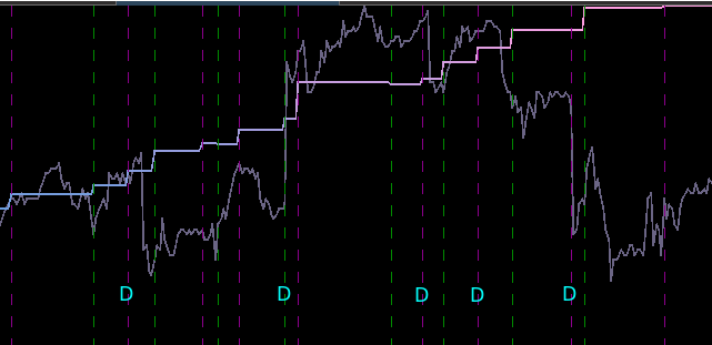
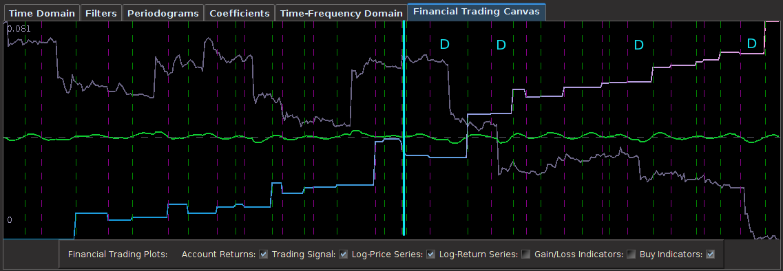
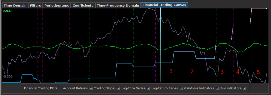
 from the band-pass design and setting the lower cutoff to 0. I also increased the smoothing parameter to $\alpha = 32$. In this newly designed filter, we see a vast improvement in the trading structure. As before, the filter was able to deduce the direction of every single close-to-open jump during the 200 out-of-sample observations, but notice that it was also able to become much more flexible in the trading during any upswing/downswing and volatile period. This is seen in more detail in Figure 7, where I added the letter ‘D’ to each of the 5 major buy/sell signals occurring before close.


 , down from
  as I had on the band-pass filter. This allows for slightly higher frequencies than

 , I then set the regularization parameters to be
  ,
, 


 = 13.2,


 , but this is typically normal and a non-issue. I had to balance for both timeliness and smoothness in this filter using both the customization parameters


 . These could be taken into account with a smart multibandpass filter in order to manifest even more trades, but I wanted to keep things simple for my first trials with high-frequency foreign exchange data. I’m quite content with the results that I’ve achieved so far.
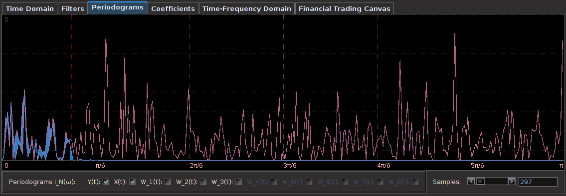


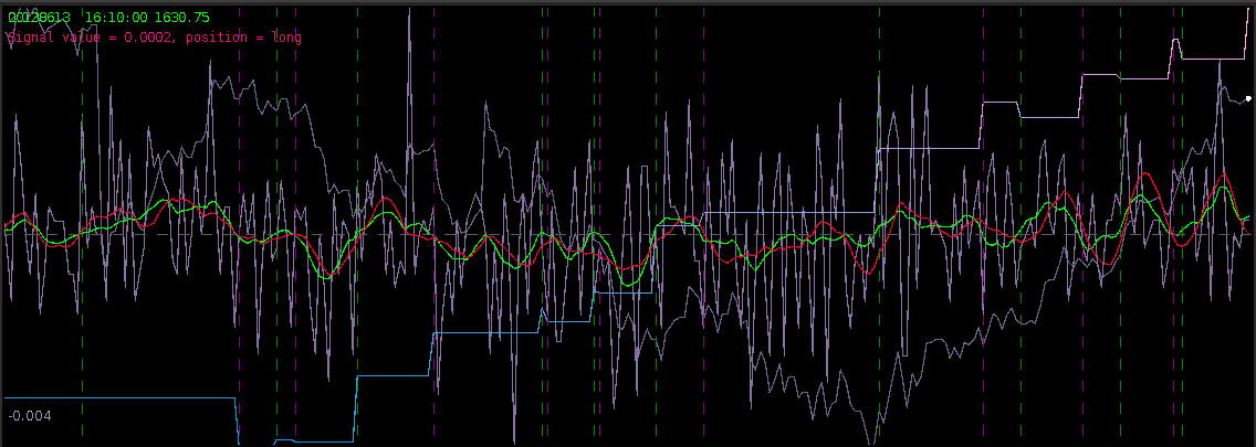
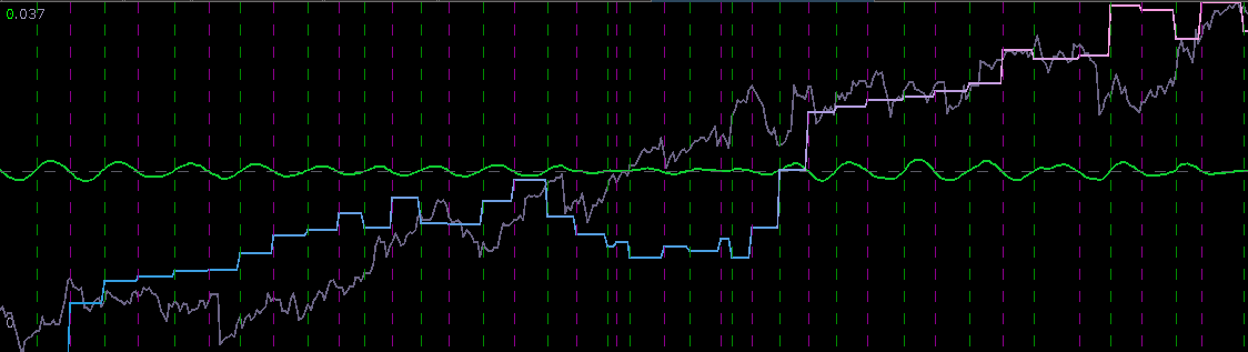
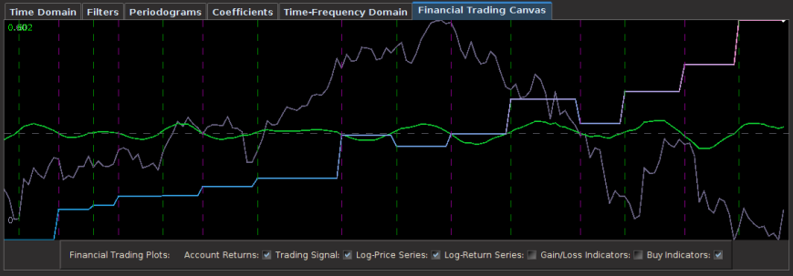
 (see my previous two articles on The Frequency Effect). Designating a lowpass or bandpass filter in the frequency domain will give an indication of what kind of patterns the extracted trading signal will trade on. Traditionally one can set a lowpass with the goal of extracting trends (with the proper amount of timeliness prioritized in the parameterization), or one can opt for a bandpass to extract smaller cyclical events for more systematic trading during volatile periods. But now suppose we could have the best of both worlds at the same time. Namely, be profitable in both steady climbs and long tumbles, while at the same time systematically hacking our way through rough sideways volatile territory, making trades at specific frequencies embedded in the share price actions not found in long trends. The answer is through the construction of multi-band pass filters. Their construction is relatively simple, but as I will demonstrate in this article with many examples, they are a bit more difficult to pinpoint optimally (but it can be done, and the results are beautiful… both aesthetically and financially).
![A := 1_{[\omega_0, \omega_1]}](https://s0.wp.com/latex.php?latex=A+%3A%3D+1_%7B%5B%5Comega_0%2C+%5Comega_1%5D%7D&bg=ffffff&fg=323232&s=0&c=20201002) ,
, ![B := 1_{[\omega_2, \omega_3]}](https://s0.wp.com/latex.php?latex=B+%3A%3D+1_%7B%5B%5Comega_2%2C+%5Comega_3%5D%7D&bg=ffffff&fg=323232&s=0&c=20201002) with
with  and
and  , zero everywhere else, it is easy to see that the motivation here is to seek a detection of both lower frequencies and low-mid frequencies in the data concurrently. With now up to four cutoff frequencies to choose from, this adds yet another few wrinkles in the degrees of freedom in parameterizing the MDFA setup. If choosing and optimizing one cutoff frequency for a simple low-pass filter in addition to customization and regularization parameters wasn’t enough, now imagine extracting signals with the addition of up to three more cutoff frequencies. Despite these additional degrees of freedom in frequency interval selection, I will later give a couple of useful hacks that I’ve found helpful to get one started down the right path toward successful extraction.
 for
for  that acts on the periodogram (or discrete Fourier transforms in multivariate mode) is now defined piecewise according to the different intervals
 ![[0,\omega_0]](https://s0.wp.com/latex.php?latex=%5B0%2C%5Comega_0%5D&bg=ffffff&fg=323232&s=0&c=20201002) ,
, ![[\omega_1, \omega_2]](https://s0.wp.com/latex.php?latex=%5B%5Comega_1%2C+%5Comega_2%5D&bg=ffffff&fg=323232&s=0&c=20201002) , and
, and ![[\omega_3, \pi]](https://s0.wp.com/latex.php?latex=%5B%5Comega_3%2C+%5Cpi%5D&bg=ffffff&fg=323232&s=0&c=20201002) . For example,
. For example,  gives a piecewise quadratic weighting function (an example shown in Figure 1) and for
  , the weighting function is piecewise linear. In practice, the piecewise power function smooths and rids of unwanted frequencies in the stop band much better than using a piecewise constant function. With these preliminaries defined, we now move on to the first steps in building and applying multiband pass filters.
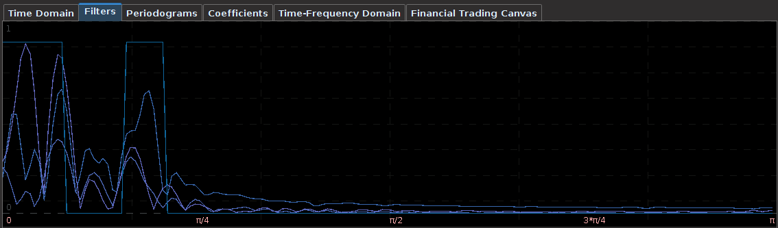
 if
if ![\omega \in [0,.17]](https://s0.wp.com/latex.php?latex=%5Comega+%5Cin+%5B0%2C.17%5D&bg=ffffff&fg=323232&s=0&c=20201002) , and 0 otherwise. This formulation, as it includes the zero frequency, should provide a local bias as well as extract very slow moving trends. The trick with these filters for building consistent trading performance is ensure a proper grip on the timeliness characteristics of the filter in a very low and narrow filter passage. Regularization and smoothness using the weighting function shouldn’t be too much of a problem or priority as typically just only a small fraction of the available degrees of freedom on the frequency domain are being utilized, so not much concern for overfitting as long as you’re not using too long of a filter. In my example, I maxed out the timeliness
, and 0 otherwise. This formulation, as it includes the zero frequency, should provide a local bias as well as extract very slow moving trends. The trick with these filters for building consistent trading performance is ensure a proper grip on the timeliness characteristics of the filter in a very low and narrow filter passage. Regularization and smoothness using the weighting function shouldn’t be too much of a problem or priority as typically just only a small fraction of the available degrees of freedom on the frequency domain are being utilized, so not much concern for overfitting as long as you’re not using too long of a filter. In my example, I maxed out the timeliness  regularization parameter to .3. Fortunately, no optimization of any parameter was needed in this example, as the performance was spiffy enough nearly right after gauging the timeliness parameter
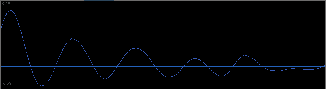
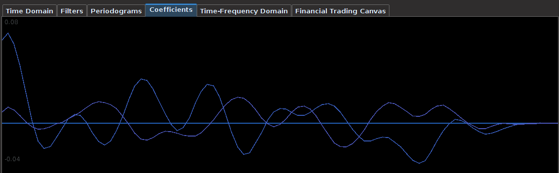
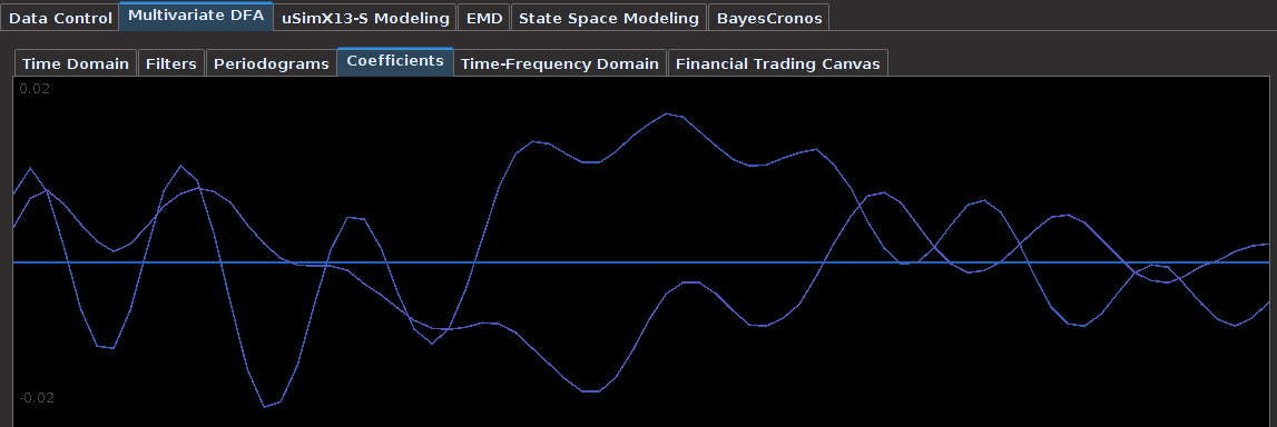
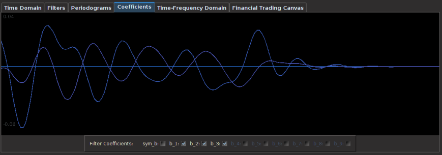
 for both the sets of explanatory log-return data and Figure 4 depicts the coefficients for the filter. Notice that in the coefficients plot, much more weight is being assigned to past values of the log-return data with extreme (min and max values) at around lags 15 and 30 for the GOOG coefficients (blue-ish line). The coefficients are also quite smooth due to the slight amount of smooth regularization imposed.

 is highly dependent on the data and should be located through a priori investigations (as I did above, without the additional bandpass).
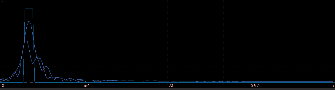
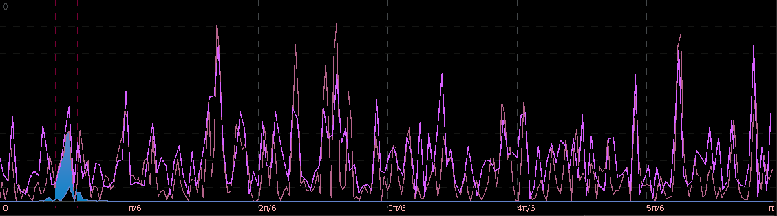
 . The largest of these peaks will be defined from here on out as the principal spectral peak (PSP). Figure 6 shows an example of an averaged periodogram of the log-return for GOOG and AAPL with the PSP indicated. You might note that there exists a much larger spectral peak located at
  , but no need to worry about that one (unless you really enjoy transaction costs). I locate this PSP as a starting point for where I want my signal to trade.
![[.49,.65]](https://s0.wp.com/latex.php?latex=%5B.49%2C.65%5D&bg=ffffff&fg=323232&s=0&c=20201002) with the PSP directly under it. I then optimized the regularization controls in-sample (a feature I haven’t discussed yet) and slightly tweaked the timeliness parameter (ended up setting it to 3) and my result (drumroll…) is shown in Figure 6.
with the PSP directly under it. I then optimized the regularization controls in-sample (a feature I haven’t discussed yet) and slightly tweaked the timeliness parameter (ended up setting it to 3) and my result (drumroll…) is shown in Figure 6.
![[.51, .68]](https://s0.wp.com/latex.php?latex=%5B.51%2C+.68%5D&bg=ffffff&fg=323232&s=0&c=20201002) , with the PSP still underneath the bandpass, but now catching on to a few more higher frequencies then before. I also slightly increased the length of the filter to see if that had any affect. After optimizing on the timeliness parameter
, with the PSP still underneath the bandpass, but now catching on to a few more higher frequencies then before. I also slightly increased the length of the filter to see if that had any affect. After optimizing on the timeliness parameter 


![(\omega_0, \omega_1) \subset [0,\pi]](https://s0.wp.com/latex.php?latex=%28%5Comega_0%2C+%5Comega_1%29+%5Csubset+%5B0%2C%5Cpi%5D&bg=ffffff&fg=323232&s=0&c=20201002) where
where  . We can introduce a constraint on the filter coefficients so as to impose a vanishing time-shift at frequency zero. As Wildi says on page 24 of the Elements paper: “A vanishing time-shift is highly desirable because turning-points in the filtered series are concomitant with turning-points in the original data.” In fact, we can take this a step further and even impose an arbitrary time-shift with the value
  at frequency zero, where
  at zero is
  , which implies
  .
.


![\omega \in [0,\pi]](https://s0.wp.com/latex.php?latex=%5Comega+%5Cin+%5B0%2C%5Cpi%5D&bg=ffffff&fg=323232&s=0&c=20201002) controls the frequency content of the output signal through the computation of the optimal filter coefficients. Defining
controls the frequency content of the output signal through the computation of the optimal filter coefficients. Defining 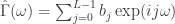 for some collection of filter coefficients
  , recall that in the plain-vanilla (univariate) direct filter approach (for ‘quasi’ stationary data), we seek to find the
  coefficients such that
  is minimized, where
  is a ‘smart’ weighting function that approximates the ‘true’ spectral density of the data (in general the periodogram of the data, or a function using the periodogram of the data). By defining
 ![[0,\pi]](https://s0.wp.com/latex.php?latex=%5B0%2C%5Cpi%5D&bg=ffffff&fg=323232&s=0&c=20201002) and zero elsewhere, we pinpoint exotic frequencies where we wish our filter to extract the features of the data. The characteristics of the generated output signal (after the resulting filter has been applied to the data) are those intrinsic to the selected frequencies in the data. The characteristics found at other frequencies are (in a perfect world) disregarded from the output signal. As we show in this article, the selection of the frequencies when defining
and zero elsewhere, we pinpoint exotic frequencies where we wish our filter to extract the features of the data. The characteristics of the generated output signal (after the resulting filter has been applied to the data) are those intrinsic to the selected frequencies in the data. The characteristics found at other frequencies are (in a perfect world) disregarded from the output signal. As we show in this article, the selection of the frequencies when defining  by changes of .01. The second method uses two different slider bars to change the values of the numerator
  and denominator
  where
where  , a form commonly used for defining different cycles in the data. The third method is to simply type in the value of the cutoff in the designated text area and then press Enter on the keyboard, where the number must be a real number in the interval
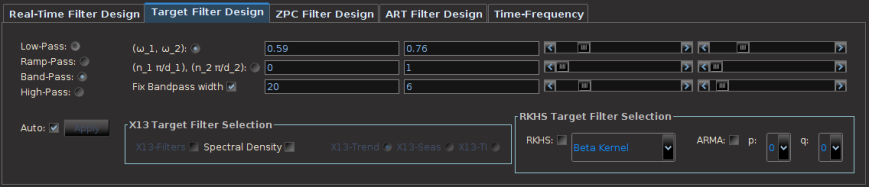
 interval to
  . Setting
  to .10-.15 is usually sufficient. Set the checkbox Fix-Bandpass width in order to secure the bandwidth of the filter.
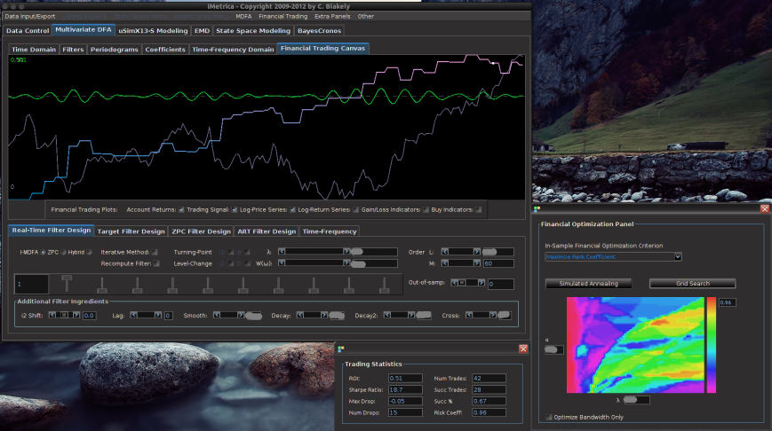
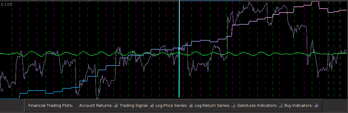
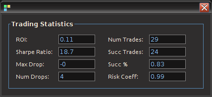
 , where the in-sample period was from 6-3-2011 to 9-21-2012. The post-optimization of the filter, showing the MDFA trading interface, the in-sample trading statistics, and the trading optimization is shown in Figure 3. Here, the in-sample maximum rank coefficient was found to be at .96 (1.0 is the best, -1.0 is pitiful), where the trade success ratio is around 67 percent, a return-on-investment at 51 percent, and a maximum loss during the in-sample period at around 5 percent. Applying this filter out-of-sample on incoming data for 30 trading days, without any adjustments to the filter, we see that the performance of the signal was very much akin to the performance in-sample (see Figure 5). At the end of the 30 out-of-sample trading days after the in-sample period, the trading signal gives a 65 percent return for a total of a 14 percent return-on-investment in 30 trading days. During this period, there were 6 trades made (3 buys and 3 sell shorts), and 5 of them were successful (with a .1 percent transaction cost for any trade), which amounts to, on average, one trade per week.