
Animation of the out-of-sample performance of one of the multibandpass filters built in this article for the daily returns of the price of Google. The resulting trading signal was extracted and yielded a trading performance near 39 percent ROI during an 80 day out-of-sample period on trading shares of Google.
To conclude the trilogy on this recent voyage through various variations on frequency domain configurations and optimizations in financial trading using MDFA and iMetrica, I venture into the world of what I call multi-bandpass filters that I recently implemented in iMetrica. The motivation of this latest endeavor in highlighting the fundamental importance of the spectral frequency domain in financial trading applications was wanting to gain better control of extracting signals and engineering different trading strategies through many different types of market movement in financial assets. There are typically four different basic types of movement a price pattern will take during its fractalesque voyage throughout the duration that an asset is traded on a financial market. These patterns/trajectories include
- steady up-trends in share price
- low volatility sideways patterns (close to white noise)
- highly volatile sideways patterns (usually cyclical)
- long downswings/trends in share price.
Using MDFA for signal extraction in financial time series, one typically indicates an a priori trading strategy through the design of the extractor, namely the target function 
With the multi-bandpass defined as two separate bands given by ![A := 1_{[\omega_0, \omega_1]}](https://s0.wp.com/latex.php?latex=A+%3A%3D+1_%7B%5B%5Comega_0%2C+%5Comega_1%5D%7D&bg=ffffff&fg=323232&s=0&c=20201002)
![B := 1_{[\omega_2, \omega_3]}](https://s0.wp.com/latex.php?latex=B+%3A%3D+1_%7B%5B%5Comega_2%2C+%5Comega_3%5D%7D&bg=ffffff&fg=323232&s=0&c=20201002)


With this multi-bandpass definition for 


![[0,\omega_0]](https://s0.wp.com/latex.php?latex=%5B0%2C%5Comega_0%5D&bg=ffffff&fg=323232&s=0&c=20201002)
![[\omega_1, \omega_2]](https://s0.wp.com/latex.php?latex=%5B%5Comega_1%2C+%5Comega_2%5D&bg=ffffff&fg=323232&s=0&c=20201002)
![[\omega_3, \pi]](https://s0.wp.com/latex.php?latex=%5B%5Comega_3%2C+%5Cpi%5D&bg=ffffff&fg=323232&s=0&c=20201002)


Figure 1: Plot of the Piecewise Smoothing Function for alpha = 15 on a mutli-band pass filter.
To motivate this newly customized approach to building financial trading signals, I begin with a simple example where I build a trading signal for the daily share price of Google. We begin with a simple lowpass filter defined by 
![\omega \in [0,.17]](https://s0.wp.com/latex.php?latex=%5Comega+%5Cin+%5B0%2C.17%5D&bg=ffffff&fg=323232&s=0&c=20201002)


Figure 2: The in-sample and out-of-sample gains made by constructing a low-pass filter employing a very high timeliness parameter and small amount of regularization in smoothness. The out-of-sample gains are nearly 30 percent and no losses on any trades.
Although not perfect, the trading signal produces a monotonic performance both in-sample and out-of-sample, which is exactly what you strive for when building these trend signals for trading. The performance out-of-sample is also highly consistent (in regards to trading frequency and no losses on any trades) with the in-sample performance. With only 4 trades being made, they were done at very interesting points in the trajectory of the Google share price. Firstly, notice that the local bias in the largest upswing is accounted for due to the inclusion of frequency zero in the low pass filter. This (positive) local bias continues out-of-sample until, interestingly enough, two days before one of the largest losses in the share price of Google over the past couple years. A slightly earlier exit out of this long position (optimally at the peak before the down turn a few days before) would have been more strategic; perhaps further tweaking of various parameters would have achieved this, but I happy with it for now. The long position resumes a few days after the dust settles from the major loss, and the local bias in the signal helps once again (after trade 2). The next few weeks sees shorter downtrending cyclical effects, and the signal fortunately turns positively increasingly right before another major turning point for an upswing in the share price. Finally, the third transaction ends the long position at another peak (3), perfect timing. The fourth transaction (no loss or gain) was quickly activated after the signal saw another upturn, and thus is now in the long position (hint: Google trending upward). Figure 3 shows the transfer functions 

Figure 3: Transfer functions for the concurrent trend filter applied to GOOG.

Figure 4: The filter coefficients for the log-return data.
Now suppose we wish to extract a trading signal that performs like a trend signal during long sweeping upswings or downswings, and at the same time shares the property that it extracts smaller cyclical swings during a sideways or highly volatile period. This type of signal would be endowed with the advantage that we could engage in a long position during upswings, trade systematically during sideways and volatile times, and on the same token avoid aggressive long-winded downturns in the price. Financial trading can’t get more optimistic then that, right? Here is where the magic of the multi-bandpass comes in. I give my general “how-to” guidelines in the following paragraphs as a step-by-step approach. As a forewarning, these signals are not easy to build, but with some clever optimization and patience they can be done.
In this new formulation, I envision not only being able to extract a local bias embedded in the log-return data but also gain information on other important frequencies to trade on while in sideways markets. To do this, I set up the lowpass filter as I did earlier on 

Click on the Animation 2: Example of constructing a multiband pass using the Target Filter control panel in iMetrica. Initially, a low-pass filter is set, then the additional bandpass is added by clicking “Multi-Pass” checkbox. The location is then moved to the desired location using the scrollbars. The new filters are computed automaticall if “Auto” is checked on (lower left corner).
Before setting any parameterization regarding customization, regularization, or filter constraints, I perform a quick scan of the periodogram (averaged periodogram if in multivariate mode) to locate what I call principal trading frequencies in the data. In the averaged periodogram, these frequencies are located at the largest spectral peaks, with the most useful ones for our purposes of financial trading typically before 


Figure 5: Principal spectral peak in the log-return data of GOOG and AAPL.
In the next step, I place a bandpass of width around .15 so that the PSP is dead-centered in the bandpass. Fortunately with iMetrica, this is a seamlessly simple task with just the use of a scrollbar to slide the positioning of this bandpass (and also adjust the lowpass) to where I desire. Animation 2 above (click on it to see the animation) shows this process of setting a multi-passband in the MDFA Target Filter control panel. Notice as I move the controls for the location of the bandpass, the filter is automatically recomputed and I can see the changes in the frequency response functions
With the bandpass set along with the lowpass, we can now view how the in-sample performance is behaving at the initial configuration. Slightly tweaking the location of the bandpass might be necessary (width not so much, in my experience between .15 and .20 is sufficient). The next step in this approach is now to not only adjust for the location of the bandpass while keeping the PSP located somewhat centered, but also adding the effects of regularization to the filter as well. With this additional bandpass, the filter has a tendency to succumb to overfitting if one is not careful enough.
In my first filter construction attempt, I placed my bandpass at ![[.49,.65]](https://s0.wp.com/latex.php?latex=%5B.49%2C.65%5D&bg=ffffff&fg=323232&s=0&c=20201002)

Figure 6: The trading performance and signal for the initial attempt at a building a multiband pass fitler.
Not bad for a first attempt. I was actually surprised at how few trades there were out-of-sample. Although there are no losses during the 80 days out-of-sample (after cyan line), and the signal is sort of what I had in mind a priori, the trades are minimal and not yielding any trading action during the period right after the large loss in Google when the market was going sideways and highly volatile. Notice that the trend signal gained from the lowpass filter indeed did its job by providing the local bias during the large upswing and then selling directly at the peak (first magenta dotted line after the cyan line). There are small transactions (gains) directly after this point, but still not enough during the sideways market after the drop. I needed to find a way to tweak the parameters and/or cutoff to include higher frequencies in the transactions.
In my second attempt, I kept the regularization parameters as they were but this time increased the bandpass to the interval ![[.51, .68]](https://s0.wp.com/latex.php?latex=%5B.51%2C+.68%5D&bg=ffffff&fg=323232&s=0&c=20201002)

Figure 7: The trading performance and signal for the second attempt at construction a multiband pass filter. This one included a few more higher frequencies.
Upon inspection, this signal behaves more consistently with what I had in mind. Notice that directly out-of-sample during the long upswing, the signal (barely) shows signs of the local bias, but enough not to make any trades fortunately. However, in this signal, we see that filter is much too late in detecting the huge loss posted by Google, and instead sells immediately after (still a profit however). Then during the volatile sideways market, we see more of what we were wishing for; timely trades to the earn the signal a quick 9 percent in the span of a couple weeks. Then the local bias kicks in again and we see not another trade posted during this short upswing, taking advantage of the local trend. This signal earned a near 22 percent ROI during the 80 day out-of-sample trading period, however not as good as the previous signal at 32 percent ROI.
Now my priority was to find another tweak that I could perform to change the trading structure even more. I’d like it to be even more sensitive to quick downturns, but at the same time keep intact the sideways trading from the signal in Figure 7. My immediate intuition was to turn on the i2 filter constraint and optimize the time-shift, similar to what I did in my previous article, part deux of the Frequency Effect. I also lessened the amount of smoothing from my weighting function

Figure 8: Third attempt at building a multiband pass filter. Here, I turn on i2 filter constraint and optimize the time shift.
While the consistency with the in-sample performance to out-of-sample performance is somewhat less than my previous attempts, out-of-sample performs nearly exactly how I envisioned. There are only two small losses of less than 1 percent each, and the timeliness of choosing when to sell at the tip of the peak in the share price of Google couldn’t have been better. There is systematic trading governed by the added multiband pass filter during the sideways and slight upswing toward the end. Some of the trades are made later than what would be optimal (the green lines enter a long position, magenta sells and enters short position), but for the most part, they are quite consistent. It’s also very quick in pinpointing its own erronous trades (namely no huge losses in-sample or out of sample). There you have it, a near monotonic performance out-of-sample with 39 percent ROI.
In examining the coefficients of this filter in Figure 9, we see characteristics of a trend filter as coefficients are largely weighting the middle lags much more than than initial or end lags (note that no decay regularization was added to this filter, only smoothness) . While at the same time however, the coefficients also weight the most recent log-return observations unlike the trend filter from Figure 4, in order to extract signals for the more volatile areas. The undulating patterns also assist in obtaining good performance in the cyclical regions.
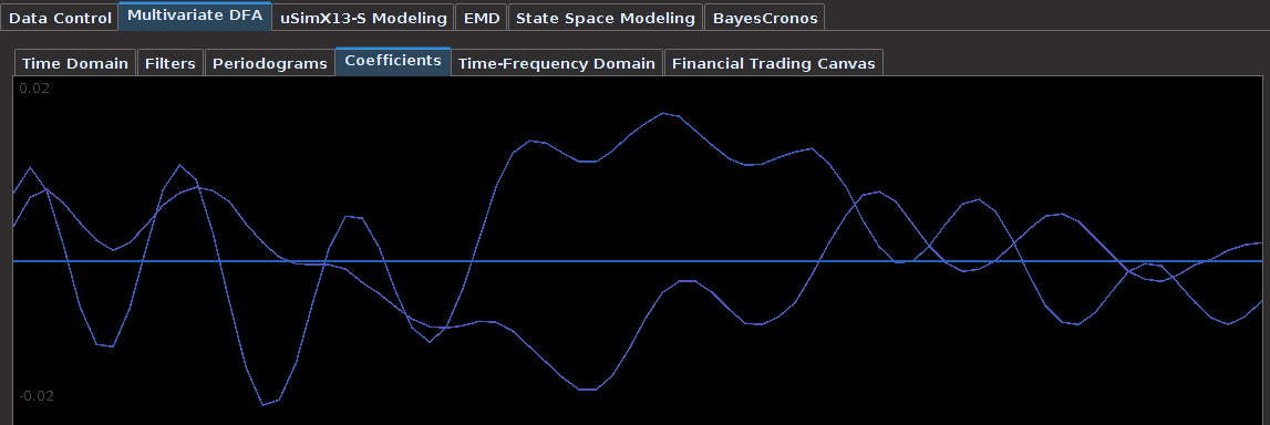
Figure 9: The coefficients of the final filter depicting characteristics of both a trend and bandpass filter, as expected.
Finally, the frequency response functions of the concurrent filters show the effect of including the PSP in the bandpass (figure 10). Notice, the largest peak in the bandpass function is found directly at the frequency of the PSP, ahh the PSP. I need to study this frequency with more examples to get a more clear picture to what it means. In the meantime, this is the strategy that I would propose. If you have any questions about any of this, feel free to email me. Until next time, happy extracting!

Figure 10: The frequency response functions of the multi-bandpass filter.

Pingback: TWS-iMetrica: The Automated Intraday Financial Trading Interface Using Adaptive Multivariate Direct Filtering | Hybrid Signal Extraction, Forecasting, and Financial Trading