iMetrica for Linux Ubuntu 64 now available

The MDFA real-time signal extraction module

The MDFA real-time signal extraction module

My first open-source release of iMetrica for Linux Ubuntu 64 can now be downloaded at my Github, with a Windows 64 version soon to follow. iMetrica is a fast, interactive, GUI-oriented software suite for predictive modeling, multivariate time series analysis, real-time signal extraction, Bayesian financial econometrics, and much more.

The principal use of iMetrica is to provide an interactive environment for the numerical and visual analysis of (multivariate) time series modeling, real-time filtering, and signal extraction. The interactive features in iMetrica boast a modeling and graphics environment for analysts, practitioners, and students of econometrics, finance, and real-time data analysis where no coding or modeling experience is necessary. All the system needs is data which can be piped into the system in many forms, including .csv, .txt, Google/Yahoo Finance, Quandle, .RData, and more. A module for connecting to MySQL databases is currently being developed. One can also simulate their own data from a one or a combination of several different popular data generating models.

With the design intending to be interactive and self-enclosed, one can change modeling data/parameter inputs and see the effects in both graphical and numerical form automatically. This feature is designed to help understand the underlying mechanics of the modeling or filtering process. One can test many attributes of the modeling or filtering process this way both visually and numerically such as sensitivity, nonlinearity, goodness-of-fit, any overfitting issues, stability, etc.

All the computational libraries were written in GNU C and/or Fortran and have been provided as Native libraries to the Java platform via JNI, where Java provides the user-interface, control, graphics, and several other components in a module format, and where each module specializes in a different data analysis paradigm. The modules available in this open-source version of iMetrica are as follows:

1) Data simulation, modeling and fitting using several popular econometric models

  • (S)ARIMA, (E)GARCH, (Multivariate) Factor models, Stochastic Volatility, High-frequency volatility models, Cycles/Trends, and more
  • Random number generators from several different types of parameterized distributions to create shocks, outliers, regression components, etc.
  • Visualize in real-time all components of the modeling process

2) An interactive GUI for multivariate real-time signal extraction using the multivariate direct filter approach (MDFA)

  • Construct mulitvariate MA filter designs, classical ARMA ZPA filtering designs, or hybrid filtering designs.
  • Analyze all components of the filtering and signal extraction process, from time-delay and smoothing control, to regularization.
  • Adaptive real-time filtering
  • Construct financial trading signals and forecasts
  • Includes a real-time/frequency analysis module using MDFA

3) An interactive GUI for X-13-ARIMA-SEATS called uSimX13

  • Perform automatic seasonal adjustment on thousands of economic time series
  • Compare SARIMA model choices using several different novel signal extraction diagnostics and tools available only in iMetrica
  • Visualize in real-time several components of modeling process
  • Analyze forecasts and compare with other models
  • All of the most important features of X-13-ARIMA-SEATS included

4) An interactive GUI for RegComponent (State Space and Unobserved Component Models)

  • Construct unobserved signal components and time-varying regression components
  • Obtain forecasts automatically and compare with other forecasting models

5) Empirical Mode Decomposition

  • Applies a fast adaptive EMD algorithm to decompose nonlinear, nonstationary data into a trend and instrinsic modes.
  • Visualize all time-frequency components with automatically generated 2D heat maps.

6) Bayesian Time Series Modeling of ARIMA, (E)GARCH, Multivariate Stochastic Volatility, HEAVY models

  • Compute and visualize posterior distribtions for all modeling parameters
  • Easily compare different model dimensions

7) Financial Trading Strategy Engineering with MDFA

  • Construct financial trading signals in the MDFA module and backtest the strategies on any frequency of data
  • Perform analysis of the strategies using forward-walk schemes
  • Automatically optimize certain components of the signal extraction on in-sample data.
  • Features a toolkit for minimizing probability of backtest overfit

Tutorials on how to use iMetrica can be found on this blog and will be added on a weekly basis, with new tools, features, and modules being added and improved on a consistent basis.

Please send any bug reports, comments, complaints, to clisztian@gmail.com.

TWS-iMetrica: The Automated Intraday Financial Trading Interface Using Adaptive Multivariate Direct Filtering

Figure 1: The TWS-iMetrica automated financial trading platform. Featuring fast performance optimization, analysis, and trading design features unique to iMetrica for building direct real-time filters to generate automated trading signals for nearly any tradeable financial asset. The system was built using Java, C, and the Interactive Brokers IB API in Java.

Figure 1: The TWS-iMetrica automated financial trading platform. Featuring fast performance optimization, analysis, and trading design features unique to iMetrica for building direct real-time filters to generate automated trading signals for nearly any tradeable financial asset. The system was built using Java, C, and the Interactive Brokers IB API in Java.

Introduction

I realize that I’ve been MIA (missing in action for non-anglophones) the past three months on this blog, but I assure you there has been good reason for my long absence. Not only have I developed a large slew of various optimization, analysis, and statistical tools in iMetrica for constructing high-performance financial trading signals geared towards intraday trading which I will (slowly) be sharing over the next several months (with some of the secret-sauce-recipes kept to myself and my current clients of course), but I have also built, engineered, tested, and finally put into commission on a daily basis the planet’s first automated financial trading platform completely based on the recently developed FT-AMDFA (adaptive multivariate direct filtering approach for financial trading). I introduce to you iMetrica’s little sister, TWS-iMetrica.

Coupled with the original software I developed for hybrid econometrics, time series analysis, signal extraction, and multivariate direct filter engineering called iMetrica, the TWS-iMetrica platform was built in a way to provide an easy to use yet powerful, adaptive, versatile, and automated trading machine for intraday financial trading with a variety of options for building your own day trading strategies using MDFA based on your own financial priorities.  Being written completely in Java and gnu c, the TWS-iMetrica system currently uses the Interactive Brokers (IB) trading workstation (TWS) Java API in order to construct the automated trades, connect to the necessary historical data feeds, and provide a variety of tick data. Thus in order to run, the system will require an activated IB trading account. However, as I discuss in the conclusion of this article, the software was written in a way to be seamlessly adapted to any other brokerage/trading platform API, as long as the API is available in Java or has Java wrappers available.

The steps for setting up and building an intraday financial trading environment using iMetrica + TWS-iMetrica are easy. There are four of them. No technical analysis indicator garbage is used here, no time domain methodologies, or stochastic calculus. TWS-iMetrica is based completely on the frequency domain approach to building robust real-time multivariate filters that are designed to extract signals from tradable financial assets at any fixed observation of frequencies (the most commonly used in my trading experience with FT-AMDFA being 5, 15, 30, or 60 minute intervals). What makes this paradigm of financial trading versatile is the ability to construct trading signals based on your own trading priorities with each filter designed uniquely for a targeted asset to be traded. With that being said, the four main steps using both iMetrica and TWS-iMetrica are as follows:

  1. The first step to building an intraday trading environment is to construct what I call an MDFA portfolio (which I’ll define in a brief moment). This is achieved in the TWS-iMetrica interface that is endowed with a user-friendly portfolio construction panel shown below in Figure 4.
  2. With the desired MDFA portfolio, selected, one then proceeds in connecting TWS-iMetrica to IB by simply pressing the Connect button on the interface in order to download the historical data (see Figure 3).
  3. With the historical data saved, the iMetrica software is then used to upload the saved historical data and build the filters for the given portfolio using the MDFA module in iMetrica (see Figure 2). The filters are constructed using a sequence of proprietary MDFA optimization and analysis tools. Within the iMetrica MDFA module, three different types of filters can be built 1) a trend filter that extracts a fast moving trend 2) a band-pass filter for extracting local cycles, and 3) A multi-bandpass filter that extracts both a slow moving trend and local cycles simultaneously.
  4. Once the filters are constructed and saved in a file (a .cft file), the TWS-iMetrica system is ready to be used for intrady trading using the newly constructed and optimized filters (see Figure 6).
Figure 4: The iMetrica MDFA module for constructing the trading filters. Features dozens of design, analysis, and optimization components to fit the trading priorities of the user and is used in conjunction with the TWS-iMetrica interface.

Figure 2: The iMetrica MDFA module for constructing the trading filters. Features dozens of design, analysis, and optimization components to fit the trading priorities of the user and is used in conjunction with the TWS-iMetrica interface.

In the remaining part of this article, I give an overview of the main features of the TWS-iMetrica software and how easily one can create a high-performing automated trading strategy that fits the needs of the user.

The TWS-iMetrica Interface

The main TWS-iMetrica graphical user interface is composed of several components that allow for constructing a multitude of various MDFA intraday trading strategies, depending on one’s trading priorities. Figure 3 shows the layout of the GUI after first being launched. The first component is the top menu featuring TWS System, some basic TWS connection variables which, in most cases, these variables are left in their default mode, and the Portfolio menu. To access the main menu for setting up the MDFA trading environment, click Setup MDFA Portfolio under the Portfolio menu. Once this is clicked, a panel is displayed (shown in Figure 4) featuring the required a priori parameters for building the MDFA trading environment that should all be filled before MDFA filter construction and trading is to take place. The parameters and their possible values are given below Figure 4.

Figure 3 - The TWS-iMetrica interface when first launched and everything blank.
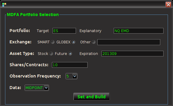
Figure 3 – The TWS-iMetrica interface when first launched and everything blank.

The Setup MDFA Portfolio panel featuring all the setting necessary to construct the automated trading MDFA environment.

Figure 4 – The Setup MDFA Portfolio panel featuring all the setting necessary to construct the automated trading MDFA environment.

  1. Portfolio – The portfolio is the basis for the MDFA trading platform and consists of two types of assets 1) The target asset from which we construct the trading signal, engineer the trades, and use in building the MDFA filter 2) The explanatory assets that provide the explanatory data for the target asset in the multivariate filter construction. Here, one can select up to four explanatory assets.
  2. Exchange – The exchange on which the assets are traded (according to IB).
  3. Asset Type – If the input portfolio is a selection of Stocks or Futures (Currencies and Options soon to be available).
  4. Expiration – If trading Futures, the expiration date of the contract, given as a six digit number of year then month (e.g. 201306 for June 2013).
  5. Shares/Contracts – The number of shares/contracts to trade (this number can also be changed throughout the trading day through the main panel).
  6. Observation frequency – In the MDFA financial trading method, we consider uniformly sampled observations of market data on which to do the trading (in seconds). The options are 1, 2, 3, 5, 15, 30, and 60 minute data. The default is 5 minutes.
  7. Data – For the intraday observations, determines the nature of data being extracted. Valid values include TRADES, MIDPOINT, BID, ASK, and BID_ASK. The default is MIDPOINT
  8. Historical Data – Selects how many days are used to for downloading the historical data to compute the initial MDFA filters. The historical data will of course come in intervals chosen in the observation frequency.

Once all the values have been set for the MDFA portfolio, click the Set and Build button which will first begin to check if the values entered are valid and if so, create the necessary data sets for TWS-iMetrica to initialize trading. This all must be done while TWS-iMetrica is connected to IB (not set in trading mode however). If the build was successful, the historical data of the desired target financial asset up to the most recent observation in regular market trading hours will be plotted on the graphics canvas. The historical data will be saved to a file named (by default) “lastSeriesData.dat” and the data will be come in columns, where the first column is the date/time of the observation, the second column is the price of the target asset, and remaining columns are log-returns of the target and explanatory data. And that’s it, the system is now setup to be used for financial trading. These values entered in the Setup MDFA Portfolio will never have to be set again (unless changes to the MDFA portfolio are needed of course).

Continuing on to the other controls and features of TWS-iMetrica, once the portfolio has been set, one can proceed to change any of the settings in main trading control panel. All these controls can be used/modified intraday while in automated MDFA trading mode. In the left most side of the panel at the main control panel (Figure 5) of the interface includes a set of options for the following features:

Figure 7 - The main control panel for choosing and/or modifying all the options during intraday trading.

Figure 5 – The main control panel for choosing and/or modifying all the options during intraday trading.

  1. In contracts/shares text field, one enters the amount of share (for stocks) or contracts (for futures)  that one will trade throughout the day. This can be adjusted during the day while the automated trading is activated, however, one must be certain that at the end of the day, the balance between bought and shorted contracts is zero, otherwise, you risk keeping contracts or shares overnight into the next trading day.Typically, this is set at the beginning before automated trading takes place and left alone.
  2. The data input file for loading historical data. The name of this file determines where the historical data associated with the MDFA portfolio constructed will be stored. This historical data will be needed in order to build the MDFA filters. By default this is “lastSeriesData.dat”. Usually this doesn’t need to be modified.
  3. The stop-loss activation and stop-loss slider bar, one can turn on/off the stop-loss and the stop-loss amount. This value determines how/where a stop-loss will be triggered relative to the price being bought/sold at and is completely dependent on the asset being traded.
  4. The interval search that determines how and when the trades will be made when the selected MDFA signal triggers a buy/sell transaction. If turned off, the transaction (a limit order determined by the bid/ask) will be made at the exact time that the buy/sell signal is triggered by the filter. If turned on, the value in the text field next to it gives how often (in seconds) the trade looks for a better price to make the transaction. This search runs until the next observation for the MDFA filter. For example, if 5 minute return data is being used to do the trading, the search looks every seconds for 5 minutes for a better price to make the given transaction. If at the end of the 5 minute period no better price has been found, the transaction is is made at the current ask/bid price. This feature has been shown to be quite useful during sideways or highly volatile markets.

The middle of the main control panel features the main buttons for both connecting to disconnecting from Interactive Brokers, initiating the MDFA automated trading environment, as well as convenient buttons used for instantaneous buy/sell triggers that supplement the automated system. It also features an on/off toggle button for activating the trades given in the MDFA automated trading environment. When checked on, transactions according to the automated MDFA environment will proceed and go through to the IB account. If turned off, the real-time market data feeds and historical data will continue to be read into the TWS-iMetrica system and the signals according to the filters will be automatically computed, but no actual transactions/trades into the IB account will be made.

Finally, on the right hand side of the main control panel features the filter uploading and selection boxes. These are the MDFA filters that are constructed using the MDFA module in iMetrica. One convenient and useful feature of TWS-iMetrica is the ability to utilize up to three direct real-time filters in parallel and to switch at any given moment during market hours between the filters. (Such a feature enhances the adaptability of the trading using MDFA filters. I’ll discuss more about this in further detail shortly).  In order to select up to three filters simultaneously, there is a filter selection panel (shown in bottom right corner of Figure 6 below) displaying three separate file choosers and a radio button corresponding to each filter. Clicking on the filter load button produces a file dialog box from which one selects a filter (a *.cft file produced by iMetrica). Once the filter is loaded properly, on success, the name of the filter is displayed in the text box to the right, and the radio button to the left is enabled. With multiple filters loaded, to select between any of them, simply click on their respective radio button and the corresponding signal will be plotted on the plot canvas (assuming market data has been loaded into the TWS-iMetrica using the market data file upload and/or has been connected to the IB TWS for live market data feeds). This is shown in Figure 6.

Figure 5 - The TWS-iMetrica main trading interface features many control options to design your own automated MDFA trading strategies.

Figure 6 – The TWS-iMetrica main trading interface features many control options to design your own automated MDFA trading strategies.

And finally, once the historical data file for the MDFA portfolio has been created, up to three filters have been created for the portfolio and entered in the filter selection boxes, and the system is connected to Interactive Brokers by pressing the Connect button, the market and signal plot panel can then be used for visualizing the different components that one will need for analyzing the market, signal, and performance of the automated trading environment. In the panel just below the plot canvas features and array of checkboxes and radiobuttons. When connected to IB and the Start MDFA Trading has been pressed, all the data and plots are updated in real-time automatically at the specific observation frequency selected in the MDFA Portfolio setup. The currently available plots are as follows:

Figure 8 - The plots for the trading interface. Features price, log-return, account cumulative returns, signal, buy/sell lines, and up to two additional  auxiliary signals.

Figure 8 – The plots for the trading interface. Features price, log-return, account cumulative returns, signal, buy/sell lines, and up to two additional auxiliary signals.

  • Price – Plots in real-time the price of the asset being traded, at the specific observation frequency selected for the MDFA portfolio.
  • Log-returns – Plots in real-time the log-returns of the price, which is the data that is being filtered to construct the trading signal.
  • Account – Shows the cumulative returns produced by the currently chosen MDFA filter over the current and historical data period (note that this does not necessary reflect the actual returns made by the strategy in IB, just the theoretical returns over time if this particular filter had been used).
  • Buy/Sell lines – Shows dashed lines where the MDFA trading signal has produced a buy/sell transaction. The green lines are the buy signals (entered a long position) and magenta lines are the sell (entered a short position).
  • Signal – The plot of the signal in real-time. When new data becomes available, the signal is automatically computed and replotted in real-time. This gives one the ability to closely monitory how the current filter is reacting to the incoming data.
  • Aux Signal 1/2 – (If available) Plots of the other available signals produced by the (up to two) other filters constructed and entered in the system. To make either of these auxillary signals the main trading signal simply select the filter associated with the signal using the radio buttons in the filter selection panel.

Along with these plots, to track specific values of any of these plots at anytime, select the desired plot in the Track Plot region of the panel bar. Once selected, specific values and their respective times/dates are displayed in the upper left corner of the plot panel by simply placing the mouse cursor over the plot panel. A small tracking ball will then be moved along the specific plot in accordance with movements by the mouse cursor.

With the graphics panel displaying the performance in real-time of each filter, one can seamlessly switch between a band-pass filter or a timely trend (low-pass) filter according to the changing intraday market conditions. To give an example, suppose at early morning trading hours there is an unusual high amount of volume pushing an uptrend or pulling a downtrend. In such conditions a trend filter is much more appropriate, being able to follow the large-variation in log-returns much better than a band-pass filter can. One can glean from the effects of the trend filter on the morning hours of the market. After automated trading using the trend filter, with the volume diffusing into the noon hour, the band-pass filter can then be applied in order to extract and trade at certain low frequency cycles in the log-return data. Towards the end of the day, with volume continuously picking up, the trend filter can then be selected again in order to track and trade any trending movement automatically.

I am in the process of currently building an automated algorithm to “intelligently” switch between the uploaded filters according to the instantaneous market conditions (with triggering of the switching being set by volume and volatility. Otherwise, for the time being, currently the user must manually switch between different filters, if such switching is at all desired (in most cases, I prefer to leave one filter running all day. Since the process is automated, I prefer to have minimal (if any) interaction with the software during the day while it’s in automated trading mode).

Conclusion

As I mentioned earlier, the main components of the TWS-iMetrica were written in a way to be adaptable to other brokerage/trading APIs. The only major condition is that the API either be available in Java, or at least have (possibly third-party?) wrappers available in Java. That being said, there are only three main types of general calls that are made automated to the connected broker 1) retrieve historical data for any asset(s), at any given time, at most commonly used observation frequencies (e.g. 1 min, 5 min, 10 min, etc.), 2) subscribe to automatic feed of bar/tick data to retrieve latest OHLC and bid/ask data, and finally 3) Place an order (buy/sell) to the broker with different any order conditions (limit, stop-loss, market order, etc.) for any given asset.

If you are interested in having TWS-iMetrica be built for your particular brokerage/trading platform (other than IB of course) and the above conditions for the API are met, I am more than happy to be hired at certain fixed compensation, simply get in contact with me. If you are interested seeing how well the automated system has performed thus far, interested in future collaboration, or becoming a client in order to use the TWS-iMetrica platform, feel free to contact me as well.

Happy extracting!

Dynamic Adaptive Filtering and Signal Extraction

This slideshow requires JavaScript.

Introduction

Dynamic adaptive filtering is the method of updating a signal extraction process in real-time using newly provided information. This newly provided information is the next sequence of observed data, such as minute, hourly, or daily log-returns in a portfolio of financial assets, or a new set of weekly/monthly observations in a set of economic indicators. The goal is to improve the properties of the extracted signal with respect to a target (symmetric) filter and the output of past (old) signal values that are not performing as they should be (perhaps due to overfitting). In the multivariate direct filtering approach framework, it is an easily workable task to update the signal while only using the most recent information given. As a recently proposed idea by Marc Wildi last month, in this dynamic form of adaptive filtering we seek to update and improve a signal for a given multivariate time series information flow by computing a new set of filter coefficients to only a small window of the time series that features the latest observations. Instead of recomputing an entire new set of filter coefficients in-sample on the entire data set, we use a much smaller data set, say the latest \tilde{N} observations on which the older filter was applied out-of-sample which is much less than the total number of observations in the time series.

The new filter coefficients computed on this small window of new observations uses as input the filtered series from original ‘old’ filter. These new updated coefficients are then applied to the output of the old filter, leading to completely re-optimized filter coefficients and thus an optimized signal, eliminating any nasty effects due overfitting or signal ‘overshooting’ in the older filter, while at the same time utilizing new information. This approach is akin to, in a way, filtering within filtering: the idea of ‘smart’-filtering on previously filtered data for optimized control of the new signal being computed. It could also be thought of as filtering filtered data, a convolution of filters, updating the real-time signal, or, more generally, adaptive filtering. However you wish to think of it, the idea is that a new filter provides the necessary updating by correcting the signal output of the old filter, applied to data out-of-sample. A rather smart idea as we will see. With the coefficients of the old filter are kept fixed, we enter into the frequency world of the output of the ‘old’ filter to gain information on optimizing the new filter. Only the coefficients of the new updated filter are optimized, and can be optimized anytime new data becomes available. This adaptive process is dynamic in the sense that we require new information to stream in in order to update the new signal by constructing a new filter. Once the new filter is constructed, the newly adapted signal is built by first applying the old filter to the data to produce the initial (non-updated) signal from the new data, then the newly constructed filter optimized from this output is then applied to the ‘old’ signal producing the smarter updated signal. Below is an outline of this algorithm for dynamic adaptive filtering stripped of much of the mathematical details. A more in-depth look at the mathematical details of MDFA and this newly proposed adaptive filtering method can be found in section 10.1 of the Elements paper by Wildi.

Basic Algorithm

We begin with a target time series Y_t, t=1,\ldots, N from which we wish to extract a signal, and along with it a set of M explanatory time series Y_{j,t}, t=1,\ldots,N, j=1,\ldots,M that may help in describing the dynamics of our target time series Y_t. Note that in many applications, such as financial trading, we normally set Y_{1,t} = Y_t so that our target time series is included in the explanatory time series set, which makes sense since it is the only known time series to perfectly describe itself (however, not in every signal extraction applications is this a good idea. See for example the GDP filtering work of Wildi here)To extract the initial signal in the given data set (in-sample), we define a target filter \Gamma(\omega), that lives on the frequency domain \omega \in [0,\pi]. We define the architecture of the filter metric space for the initial signal extraction by the set of parameters \Theta_0 := (L, \Gamma, \alpha, \lambda, i1, i2, \lambda_{s}, \lambda_{d}, \lambda{c}), where L is the desired length of the filter, \alpha and \lambda are the smoothness and timeliness customization controls, and \lambda_{s}, \lambda_{d}, \lambda{c} are the regularization parameters for smooth, decay, and cross, respectively. Once the filter is computed, we obtain a collection of filter coefficients b^j_l, l=0,\ldots,L-1 for each explanatory time series j=1,\ldots,M. The in-sample real-time signal X_t, t = L-1,\ldots,N is then produced by applying the filter coefficients on each respective explanatory series.

Now suppose we have new information flowing. With each new observation in our explanatory series Y_{j,t}, t=N+1,\ldots, we can apply the filter coefficients b^j_l to obtain the extracted signal X_t for the real-time estimate of the desired signal at each new observation t=N+1,\ldots. This is, of course, out-of-sample signal extraction. With the new information available from say t=N+1 to t=N+\tilde{N}, we wish to update our signal to include this new information. Instead of recomputing the entire filter for the N+\tilde{N}, a smarter idea recently proposed last month by Wildi in his MDFA blog is to use the output produced by applying each individual filter coefficient set b^j_l on their respective explanatory series as input into building the newly updated filter X_{j,t} = \sum_{l=0}^L b^j_l Y_{j,t-l}. We thus create a new set of M time series X_{j,t}, t=N+1,\ldots,\tilde{N} and thus the filtered explanatory data series become the input to the MDFA solver, where we now solve for a new set of filter coefficients b^j_{l,new} to be applied on the output of the old filter of the new incoming data. In this new filter construction, we build a new architecture for the signal extraction, where a whole new set of parameters can be used \Theta_1 := (L_1, \Gamma, \tilde{\alpha}, \tilde{\lambda}, i1, i2, \tilde{\lambda}_{s}, \tilde{\lambda}_{d}, \tilde{\lambda}_{c}). This is the main idea behind this dynamic adaptive filtering process: we are building a signal extraction architecture within another signal extraction architecture since we are basing this new update design on previous signal extraction performance.  Furthermore, since a much shorter span of observations, namely \tilde{N} << N, is being used to construct the new filters, one of the advantages of this filter updating is that it is extremely fast, as well as being effective. As we will show in the next section of this article, all aspects of this dynamic adaptive filtering can be easily controlled, tested, and applied in the MDFA module of iMetrica using a new adaptive filtering control panel. One can control all aspects, from filter length to all the filter parameters in the new updated filter design, and then apply the results to out-of-sample data to compare performance.

Dynamic Adaptive Filtering Interface in iMetrica

The adaptive filtering capabilities in iMetrica are controlled by an interface that allows for adjusting all aspects of the adaptive filter, including number of observations, filter length L, customization controls for timeliness and smoothness, and controls for regularization. The process for controlling and applying dynamic adaptive filtering in iMetrica is accomplished as follows. Firstly, the following two things are required in order to perform dynamic adaptive filtering.

  1. Data. A target time series and (optional) M explanatory series that describe the target series all available on N observations for in-sample filter computation along with a stream of future information flow (i.e. an additional set of, say \tilde{N}, future observations for each of the M + 1 series.
  2. An initial set of optimized filter coefficients b^j_l for the signal of the data in-sample.

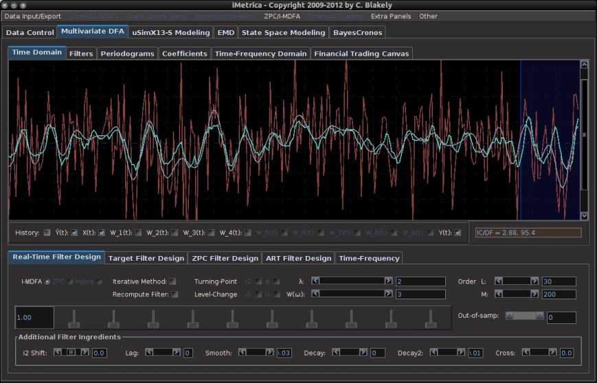
With these two prerequisites, we are now ready to test different dynamic adaptive filtering strategies. Figure 1 shows the MDFA module interface with time series data of a target series (shown in red) and four explanatory series (not plotted). Using the parameter configuration shown in Figure 1, an initial filter for computing the signal (green plot) that has been optimized in-sample on 300 observations of data and then applied to 30 out-of-sample observations (shown in the blue shaded region). As these final 30 observations of the signal have been produced using 30 out-of-sample observations, we can take note of its out-of-sample performance. Here, the performance of the signal has much room to improve. In this example, we use simulated data (conditionally heteroskedastic data generating process to emulate log-return type data) so that we are able to compare the computed updated signals with a high-order approximation of the target symmetric “perfect” signal (shown in gray in Figure 1).

The original signal (green) built using 300 observations in-sample, and then applied to 30 out-of-sample observations. A high-order approximation to the target symmetric filter is plotted in gray.

Figure 1. The original signal (green) built using 300 observations in-sample, and then applied to 30 out-of-sample observations. A high-order approximation to the target symmetric filter is plotted in gray. The blue shaded region is the region in which we wish to apply dynamic filter updating.

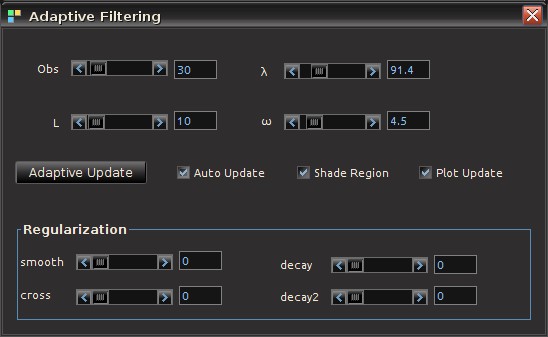
Now suppose we wish to improve performance of the signal in future out-of-sample observations by updating the filter coefficients to produce better smoothness, timeliness, and regularization properties. The first step is to ensure that the “Recompute Filter” option is not on (the checkbox in the Real-Time Filter Design panel. This should have been done already to produce the out-of-sample signal). Then go to the MDFA menu at the top of the software and click on “Adaptive Update”. This will pop open the Adaptive Filtering control panel from which we control everything in the new filter updating coefficients (see Figure 2).

The panel interface for controlling every aspect of updating a filter.

Figure 2. The panel interface for controlling every aspect of updating a filter in real-time.

The controls on the Adaptive Filtering panel are explained as follows:

  • Obs. Sets the number of the latest observations used in the filter update. This is normally set to however many new observations out-of-sample have been streamed into the time series since the last filter computation. Although one can certainly include observations from the original in-sample period as well by simply setting Obs to a number higher than the number of recent out-of-sample observations. The minimum amount of observations is 10 and the maximum is the total length of the time series.
  • L. Sets the length of the updating filter. Minimum is 5 and maximum is the number of observations minus 5.
  • \lambda and \alpha. The customization of timeliness and smoothness parameters for the filter construction. These controls are strictly for the updating filter and independent of the ‘old’ filter.
  • Adaptive Update. Once content with the settings of the update filter, press this button to compute the new filter and apply to the data. The results of the effects of the new filter will automatically appear in the main plotting canvas, specifically in the region of interest (shaded by blue, see blow).
  • Auto Update. A check box that, if turned on, will automatically compute the new filter for any changes in the filter parameters and automatically plots the effects of the new filter in the main plotting canvas. This is a nice option to use when visually testing the output of the new filter as one can automatically see effects from any small changes to the parameter setting of the filter. This option also renders the “Adaptive Update” button obsolete.
  • Shade Region. This check box, when activated, will shade the windowing region at the end of time series in which the updating is taking place. Provides a convenient way to pinpoint the exact region of interest for signal updating. The shaded region will appear in a dark blue shade (as shown in Figures 1, 4,6, and 7).
  • Plot Updates. Clicking this checkbox on and off will plot the newly updated signal (on position) or the older signal (off position). This is a convenient feature as one is able to easily visually compare the new updated signal with the old signal to test for its effectiveness. If adding out-of-sample data and this feature is turned on, it will also apply the new updated filter coefficients to the new data as it comes in. If in the off position, it will only apply the ‘old’ filter coefficients.
  • Regularization. All the regularization controls for the updating filter.

To update a signal in real-time, first select the number of observations \tilde{N} and the length of the filter from the Obs and L sliding scrollbars, respectively. This will be the total number of observations used in the adaptive updating. For example, when new dynamics appear in the time series out-of-sample that the original old filter was not able to capture, the filter updating should include this new information.  Click the checkbox marked Shade Region to highlight in a dark shade of blue the region in which the updated signal will be computed (this is shown in Figure 1).  When the number of observations or length of filter changes, the shaded region reflects these changes and adjusts accordingly. After the region of interest is selected, customization and regularization of the signal can then be applied using the sliding scrollbars. Click the “Auto Update” checkbox to the ‘on’ position to see the effects of the parameterization on the signal computed in the highlighted region automatically. Once content with the filter parameterization, visually comparing the new updated signal with the old signal can be achieved simply by toggling the Plot Updates checkbox. To apply this new filter configuration to out-of-sample data, simply add more out-of-sample data by clicking the out-of-sample slider scrollbar control on the Real-Time Direct Filter control panel (provided that more out-of-sample data is available). This will automatically apply the ‘old’ original filter along with the updated filter on the new incoming out-of-sample data. If not content with the updated signal, simply remove the new out-of-sample data by clicking ‘back’ in the out-of-sample scrollbar, and adjust the parameters to your liking and try again. To continuously update the signal, simply reapply the above process as new out-of-sample data is added. As long as the “Plot Updates” is turned on, the newly adapted signal will always be plotted in the windowed region of interest. See Figures 4-7 to see this process in action.

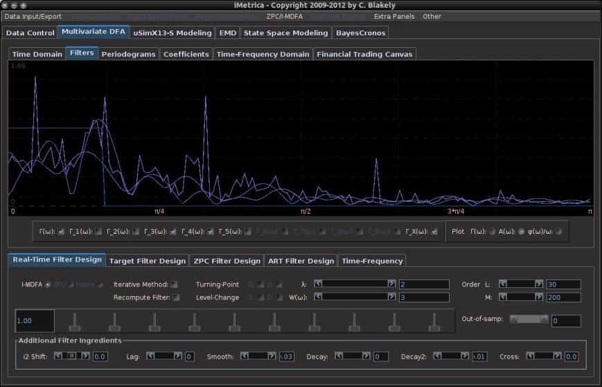
In this example,  as previously mentioned, we computed the original signal in-sample using 300 observations and then applied the filter coefficients to 30 out-of-sample observations (this was produced by checking “Recompute Filter” off).  This is plotted in Figure 4, with the blue shaded region highlighting the 30 latest observations, our region of interest. Notice a significant mangling of timeliness and signal amplification in the pass-band of the filter. This is due to bad properties of the filter coefficients. Not enough regularization was applied. Surely enough, the amplitude of the frequency response function in the original filter shows the overshooting in the pass-band (see Figure 5).  To improve this signal, we apply an adaptive update by launching the Adaptive Update menu and configuring the new filter. Figure 6 shows the updated filter in the windowed region, where we chose a combination of timeliness and light regularization. There is a significant improvement in the timeliness of the signal. Any changes in the parameterization of the filter space is automatically computed and plotted on the canvas, a huge convenience as we can easily test different parameter configurations to easily identify the signal that satisfies the priorities of the user. In the final plot, Figure 7, we have chosen a configuration with a high amount of regularization to prevent overfitting. Compared with the previous two signals in the region of interest (Figures 4 and 6), we see an even greater mollification of the unwanted amplitude overshooting in the signal, without compromising with a lack of timeliness and smoothness properties. A high-order approximation to the targeted symmetric filter is also plotted in this example for comparison convenience (since the data is simulated, we know the future data, and hence the symmetric filter).

Tune in later this week for an example of Dynamic Adaptive Filtering applied to financial trading.

Applying an update to the signal by allocating the 30 most recent out-of-sample observations and computing a new filter of length 10. The blue shaded region shows the updating region. Here the old filter has been applied to the 30 out-of-sample observations and we notice significant mangling of timeliness and signal amplification in the pass-band of the filter. This is due to bad properties of the filter coefficients. Not enough regularization was applied.

Figure 4. Plot of the signal out-of-sample before applying an update to the signal by allocating the 30 most recent out-of-sample observations and computing a new filter of length 10. The blue shaded region shows the updating region. Here the original old filter constructed in-sample has been applied to the 30 out-of-sample observations and we notice significant mangling of timeliness and signal amplification in the pass-band of the filter. This is due to bad properties of the filter coefficients. Not enough regularization was applied.

Figure 5. The overshooting in the pass-band of the frequency response function multivariate filter. The spikes above one in the pass-band indicate this and will most-likely produce overshooting in the signal out-of-sample.

Figure 5. The overshooting in the pass-band of the frequency response function multivariate filter. The spikes above one in the pass-band indicate this and will most-likely produce overshooting in the signal out-of-sample.

After filter updating in the final 30 observations. We chose the filter settings in the adaptive filter settings to improve timeliness with a small amount of smoothing. Furthermore, regularization (smooth, decay) were applied to ensure no overfitting. Notice how the properties of the signal are vastly improved (namely timeliness and little to no overshooting).

Figure 6 After filter updating in the final 30 observations. We chose the filter settings in the adaptive filter settings to improve timeliness with a small amount of smoothing. Furthermore, regularization (smooth, decay) was applied to ensure no overfitting. Notice how the properties of the signal are vastly improved (namely timeliness and little to no overshooting).

Not satisfied with the results of our filter update, we can easily adjust the parameters more to find a satisfying configuration. In this example, since the data is simulated, I've computed the symmetric filter to compare my results with the theoretically "perfect" filter. After further adjusting regularization parameters, I end up with this signal shown in the plot. Here, the gray signal is the target symmetric "perfect" signal. The result is a very close fit to the target signal with no overfitting.

Figure 7. Not satisfied with the results of our filter update, we can easily adjust the parameters more to find a satisfying configuration. In this example, since the data is simulated, I’ve computed the symmetric filter to compare my results with the theoretically “perfect” filter. After further adjusting regularization parameters, I end up with this signal shown in the plot. Here, the gray signal is a high-order approximation to the target symmetric “perfect” signal. The result is a very close fit to the target signal with no overfitting.