
Figure 1: In-sample (observations 1-250) and out-of-sample performance of the trading signal built in this tutorial using MDFA. (Top) The log price of the Yen (FXY) in 15 minute intervals and the trades generated by the trading signal. Here black line is a buy (long), blue is sell (short position). (Bottom) The returns accumulated (cash) generated by the trading, in percentage gained or lost.
In my previous article on high-frequency trading in iMetrica on the FOREX/GLOBEX, I introduced some robust signal extraction strategies in iMetrica using the multidimensional direct filter approach (MDFA) to generate high-performance signals for trading on the foreign exchange and Futures market. In this article I take a brief leave-of-absence from my world of developing financial trading signals in iMetrica and migrate into an uber-popular language used in finance due to its exuberant array of packages, quick data management and graphics handling, and of course the fact that it’s free (as in speech and beer) on nearly any computing platform in the world.
This article gives an intro tutorial on using R for high-frequency trading on the FOREX market using the R package for MDFA (offered by Herr Doktor Marc Wildi von Bern) and some strategies that I’ve developed for generating financially robust trading signals. For this tutorial, I consider the second example given in my previous article where I engineered a trading signal for 15-minute log-returns of the Japanese Yen (from opening bell to market close EST). This presented slightly new challenges than before as the close-to-open jump variations are much larger than those generated by hourly or daily returns. But as I demonstrated, these larger variations on close-to-open price posed no problems for the MDFA. In fact, it exploited these jumps and made large profits by predicting the direction of the jump. Figure 1 at the top of this article shows the in-sample (observations 1-250) and out-of-sample (observations 251 onward) performance of the filter I will be building in the first part of this tutorial.
Throughout this tutorial, I attempt to replicate these results that I built in iMetrica and expand on them a bit using the R language and the implementation of the MDFA available in here. The data that we consider are 15-minute log-returns of the Yen from January 4th to January 17th and I have them saved as an .RData file given by ld_fxy_insamp. I have an additional explanatory series embedded in the .RData file that I’m using to predict the price of the Yen. Additionally, I also will be using price_fxy_insamp which is the log price of Yen, used to compute the performance (buy/sells) of the trading signal. The ld_fxy_insamp will be used as the in-sample data to construct the filter and trading signal for FXY. To obtain this data so you can perform these examples at home, email me and I’ll send you all the necessary .RData files (the in-sample and out-of-sample data) in a .zip file. Taking a quick glance at the ld_fxy_insamp data, we see log-returns of the Yen at every 15 minutes starting at market open (time zone UTC). The target data (Yen) is in the first column along with the two explanatory series (Yen and another asset co-integrated with movement of Yen).
> head(ld_fxy_insamp)

[,1]           [,2]          [,3]

2013-01-04 13:30:00  0.000000e+00   0.000000e+00  0.0000000000

2013-01-04 13:45:00  4.763412e-03   4.763412e-03  0.0033465833

2013-01-04 14:00:00 -8.966599e-05  -8.966599e-05  0.0040635638

2013-01-04 14:15:00  2.597055e-03   2.597055e-03 -0.0008322064

2013-01-04 14:30:00 -7.157556e-04  -7.157556e-04  0.0020792190

2013-01-04 14:45:00 -4.476075e-04  -4.476075e-04 -0.0014685198
Moving on, to begin constructing the first trading signal for the Yen, we begin by uploading the data into our R environment, define some initial parameters for the MDFA function call, and then compute the DFTs and periodogram for the Yen.
load(paste(path.pgm,"ld_fxy_in15min.RData",sep=""))    #load in-sample log-returns of Yen
load(paste(path.pgm,"price_fxy_in15min.RData",sep="")) #load in-sample log-price of Yen

in_samp_lenprice_insample<-price_fxy_insamp

#setup some MDFA variables
x<-ld_fxy_insamp
len<-length(x[,1])
shift_constraint<-rep(0,length(x[1,])-1)
weight_constraint<-rep(0,length(x[1,])-1)
d<-0
plots<-T
lin_expweight<-F

# Compute DFTs and periodogram for initial analysis
spec_obj<-spec_comp(len,x,d)
weight_func<-spec_obj$weight_func
K<-length(weight_func[,1])-1
fxy_periodogram<-abs(spec_obj$weight_func[,1])^2
As I’ve mentioned in my previous articles, my step-by-step strategy for building trading signals always begin by a quick analysis of the periodogram of the asset being traded on. Holding the key to providing insight into the characteristics of how the asset trades, the periodogram is an essential tool for navigating how the extractor 


Figure 2: Periodogram of FXY (Japanese Yen) along with spectral peaks and two different frequency cutoffs.
In our first example we consider the larger frequency as the cutoff for 


After uploading both the in-sample log-return data along with the corresponding log price of the Yen for computing the trading performance, we the proceed in R to setting initial filter settings for the MDFA routine and then compute the filter using the IMDFA_comp function. This returns both the i_mdfa& object holding coefficients, frequency response functions, and statistics of filter, along with the signal produced for each explanatory series. We combine these signals to get the final trading signal in-sample. All this is all done in R as follows:
cutoff<-pi/6 #set frequency cutoff
Gamma<-((0:K)<(cutoff*K/pi)) #define Gamma

grand_mean<-F
Lag<-0
L<-82
lambda_smooth<-0
lambda_cross<-0
lambda_decay<-c(0.,0.) #regularization - decay

lambda<-0
expweight<-0
i1<-F
i2<-F
# compute the filter for the given parameter definitions
i_mdfa_obj<-IMDFA_comp(Lag,K,L,lambda,weight_func,Gamma,expweight,cutoff,i1,i2,weight_constraint,
lambda_cross,lambda_decay,lambda_smooth,x,plots,lin_expweight,shift_constraint,grand_mean)

# after computing filter, we save coefficients
bn<-i_mdfa_obj$i_mdfa$b

# now we build trading signal
trading_signal<-i_mdfa_obj$xff[,1] + i_mdfa_obj$xff[,2]
The resulting frequency response functions of the filter and the coefficients are plotted in the figure below.
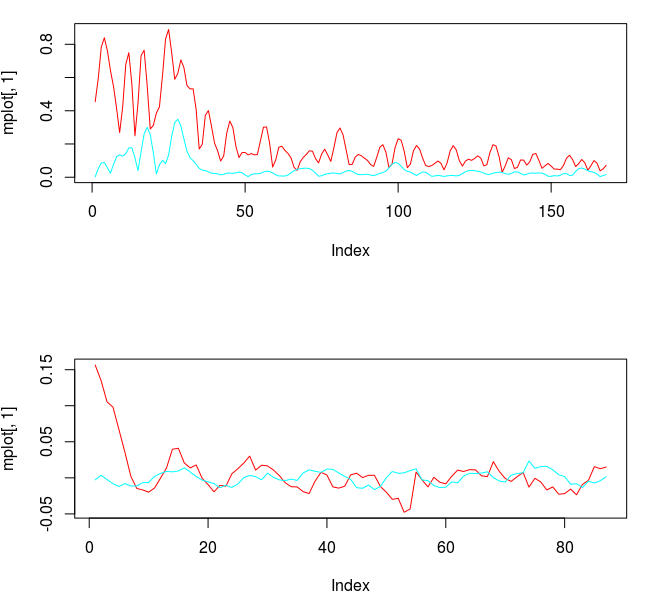
Figure 3: The Frequency response functions of the filter (top) and the filter coefficients (below)
Notice the abundance of noise still present passed the cutoff frequency. This is mollified by increasing the expweight smoothness parameter. The coefficients for each explanatory series show some correlation in their movement as the lags increase. However, the smoothness and decay of the coefficients leaves much to be desired. We will remedy this by introducing regularization parameters. Plots of the in-sample trading signal and the performance in-sample of the signal are shown in the two figures below. Notice that the trading signal behaves quite nicely in-sample. However, looks can be deceiving. This stellar performance is due in large part to a filtering phenomenon called overfitting. One can deduce that overfitting is the culprit here by simply looking at the nonsmoothness of the coefficients along with the number of freezed degrees of freedom, which in this example is roughly 174 (out of 174), way too high. We would like to get this number at around half the total amount of degrees of freedom (number of explanatory series x L).
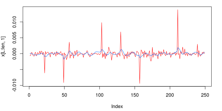
Figure 4: The trading signal and the log-return data of the Yen.
The in-sample performance of this filter demonstrates the type of results we would like to see after regularization is applied. But now comes for the sobering effects of overfitting. We apply these filter coeffcients to 200 15-minute observations of the Yen and the explanatory series from January 18 to February 1 2013 and compare with the characteristics in-sample. To do this in R, we first load the out-of-sample data into the R environment, and then apply the filter to the out-of-sample data that I defined as x_out.
load(paste(path.pgm,"ld_fxy_out15min.RData",sep=""))
load(paste(path.pgm,"price_fxy_out15min.RData",sep=""))
x_out<-rbind(ld_fxy_insamp,ld_fxy_outsamp) #bind the in-sample with out-of-sample data
xff<-matrix(nrow=out_samp_len,ncol=2)

#apply filter built in-sample
for(i in 1:out_samp_len)
{
  xff[i,]<-0
  for(j in 2:3)
  {
      xff[i,j-1]<-xff[i,j-1]+bn[,j-1]%*%x_out[335+i:(i-L+1),j]
  }
}
trading_signal_outsamp<-xff[,1] + xff[,2]     #assemble the trading signal out-of-sample
trade_outsamp<-trading_logdiff(trading_signal_outsamp,price_outsample,.0005)  #compute the performance
The plot in Figure 5 shows the out-of-sample trading signal. Notice that the signal is not nearly as smooth as it was in-sample. Overshooting of the data in some areas is also obviously present. Although the out-of-sample overfitting characteristics of the signal are not horribly suspicious, I would not trust this filter to produce stellar returns in the long run.

Figure 5 : Filter applied to 200 15 minute observations of Yen out-of-sample to produce trading signal (shown in blue)
Following the previous analysis of the mean-squared solution (no customization or regularization), we now proceed to clean up the problem of overfitting that was apparent in the coefficients along with mollifying the noise in the stopband (frequencies after
lambda_smooth<-0.63
lambda_cross<-0.
lambda_decay<-c(0.119,0.099)
lambda<-9
expweight<-8.5

i_mdfa_obj<-IMDFA_comp(Lag,K,L,lambda,weight_func,Gamma,expweight,cutoff,i1,i2,weight_constraint,
lambda_cross,lambda_decay,lambda_smooth,x,plots,lin_expweight,shift_constraint,grand_mean)

bn<-i_mdfa_obj$i_mdfa$b    #save the filter coefficients

trading_signal<-i_mdfa_obj$xff[,1] + i_mdfa_obj$xff[,2]  #compute the trading signal
trade<-trading_logdiff(trading_signal[L:len],price_insample[L:len],0) #compute the in-sample performance
Figure 6 shows the resulting frequency response function for both explanatory series (Yen in red). Notice that the largest spectral peak found directly before the frequency cutoff at

Figure 6: The frequency response functions and the coefficients after regularization and smoothing have been applied (top). The smoothed coefficients with slight decay at the end (bottom). Number of freezed degrees of freedom is approximately 102 (out of 172).
Along with an improved freezed degrees of freedom and no apparent havoc of overfitting, we apply this filter out-of-sample to the 200 out-of-sample observations in order to verify the improvement in the structure of the filter coefficients (shown below in Figure 7). Notice the tremendous improvement in the properties of the trading signal (compared with Figure 5). The overshooting of the data has be eliminated and the overall smoothness of the signal has significantly improved. This is due to the fact that we’ve eradicated the presence of overfitting.

Figure 7: Out-of-sample trading signal with regularization.
With all indications of a filter endowed with exactly the characteristics we need for robustness, we now apply the trading signal both in-sample and out of sample to activate the buy/sell trades and see the performance of the trading account in cash value. When the signal crosses below zero, we sell (enter short position) and when the signal rises above zero, we buy (enter long position).
The top plot of Figure 8 is the log price of the Yen for the 15 minute intervals and the dotted lines represent exactly where the trading signal generated trades (crossing zero). The black dotted lines represent a buy (long position) and the blue lines indicate a sell (and short position). Notice that the signal predicted all the close-to-open jumps for the Yen (in part thanks to the explanatory series). This is exactly what we will be striving for when we add regularization and customization to the filter. The cash account of the trades over the in-sample period is shown below, where transaction costs were set at .05 percent. In-sample, the signal earned roughly 6 percent in 9 trading days and a 76 percent trading success ratio.

Figure 8: In-sample performance of the new filter and the trades that are generated.
Now for the ultimate test to see how well the filter performs in producing a winning trading signal, we applied the filter to the 200 15-minute out-of-sample observation of the Yen and the explanatory series from Jan 18th to February 1st and make trades based on the zero crossing. The results are shown below in Figure 9. The black lines represent the buys and blue lines the sells (shorts). Notice the filter is still able to predict the close-to-open jumps even out-of-sample thanks to the regularization. The filter succumbs to only three tiny losses at less than .08 percent each between observations 160 and 180 and one small loss at the beginning, with an out-of-sample trade success ratio hitting 82 percent and an ROI of just over 4 percent over the 9 day interval.

Figure 9: Out-of-sample performance of the regularized filter on 200 out-of-sample 15 minute returns of the Yen. The filter achieved 4 percent ROI over the 200 observations and an 82 percent trade success ratio.
Compare this with the results achieved in iMetrica using the same MDFA parameter settings. In Figure 10, both the in-sample and out-of-sample performance are shown. The performance is nearly identical.

Figure 10: In-sample and out-of-sample performance of the Yen filter in iMetrica. Nearly identical with performance obtained in R.
Example 2
Now we take a stab at producing another trading filter for the Yen, only this time we wish to identify only the lowest frequencies to generate a trading signal that trades less often, only seeking the largest cycles. As with the performance of the previous filter, we still wish to target the frequencies that might be responsible to the large close-to-open variations in the price of Yen. To do this, we select our cutoff to be
For this new filter, we keep things simple by continuing to use the same regularization parameters chosen in the previous filter as they seemed to produce good results out-of-sample. The 

Figure 11: Frequency response functions of the two filters and their corresponding coefficients.
To test the effectiveness of this new lower trading frequency design, we apply the filter coefficients to the 200 out-of-sample observations of the 15-minute Yen log-returns. The performance is shown below in Figure 12. In this filter, we clearly see that the filter still succeeds in predicting correctly the large close-to-open jumps in the price of the Yen. Only three total losses are observed during the 9 day period. The overall performance is not as appealing as the previous filter design as less amount of trades are made, with a near 2 percent ROI and 76 percent trade success ratio. However, this design could fit the priorities for a trader much more sensitive to transaction costs.

Figure 12: Out-of-sample performance of filter with lower cutoff.
Conclusion

Verification and cross-validation is important, just as the most interesting man in the world will tell you.
The point of this tutorial was to show some of the main concepts and strategies that I undergo when approaching the problem of building a robust and highly efficient trading signal for any given asset at any frequency. I also wanted to see if I could achieve similar results with the R MDFA package as my iMetrica software package. The results ended up being nearly parallel except for some minor differences. The main points I was attempting to highlight were in first analyzing the periodogram to seek out the important spectral peaks (such as ones associate with close-to-open variations) and to demonstrate how the choice of the cutoff affects the systematic trading. Here’s a quick recap on good strategies and hacks to keep in mind.
Summary of strategies for building trading signal using MDFA in R:
- As I mentioned before, the periodogram is your best friend. Apply the cutoff directly after any range of spectral peaks that you want to consider. These peaks are what generate the trades.
- Utilize a choice of filter length
- Begin by computing the filter in the mean-square sense, namely without using any customization or regularization and see exactly what needs to be approved upon by viewing the frequency response functions and coefficients for each explanatory series. Good performance of the trading signal in-sample (and even out-of-sample in most cases) is meaningless unless the coefficients have solid robust characteristics in both the frequency domain and the lag domain.
- I recommend beginning with tweaking the smoothness customization parameter expweight and the lambda_smooth regularization parameters first. Then proceed with only slight adjustments to the lambda_decay parameters. Finally, as a last resort, the lambda customization. I really never bother to look at lambda_cross. It has seldom helped in any significant manner. Since the data we are using to target and build trading signals are log-returns, no need to ever bother with i1 and i2. Those are for the truly advanced and patient signal extractors, and should only be left for those endowed with iMetrica 😉
If you have any questions, or would like the high-frequency Yen data I used in these examples, feel free to contact me and I’ll send them to you. Until next time, happy extracting!

Hi Chris,
You say :
“Taking a quick glance at the ld_fxy_insamp data, we see log-returns of the Yen at every 15 minutes starting at market open (time zone UTC). The target data (Yen) is in the first column along with the two explanatory series (Yen and another asset co-integrated with movement of Yen).”
So in your file in input you use the log(close-returns) twice (col1 and 2) and a another asset ?
Can you tell me more about this another asset cointegred ? how you find it ?
While it’s not so obvious to determine a set of explanatory variables that will improve signal (and trading) performance, I developed a tool called fundamental frequency component analysis that helps me choose series with strong lag s correlations at certain frequencies I’m interested in. The method seems to work pretty well so far in my experience.
Thanks Chris,
have you planned other thread in the coming weeks? 😉
Yes, I have many new ideas for articles, and will be writing one soon. I’ve been busy the past couple months improving the methodology even more, making it even more robust for financial trading. The problem is I start to give away too many of my secrets and will eventually lose my competitive advantage, so I need to remain a bit cryptic
Another question :
What your favorites time frame ? 15 mins i think ?
15 minutes is a good range, the lower the frequency the better and more robust the signal will be. However, in practice I’m currently using 5 min returns with a proprietary trading firm in Chicago on Index Futures.
Chris,
You filtre the time in your data ? You trade only of 13:30pm until 20pm ?
You overnight trade ?