Dream within a dream: How science fiction concepts from the movie Inception can be accomplished in real life (via MDFA)

Posted on December 21, 2012 by Christian Dallas Blakely

“Careful, we may be in a model…within a model.” (From an Inception movie poster.)

Have you ever seen the movie Inception and wondered, “Gee, wouldn’t it be neat if I could do all that fancy subconscious dream within a dream manipulation stuff”? Well now you can (in a metaphorical way) using MDFA and iMetrica. I explain how in this article.

Before I begin, may I first draw your attention to a brief introduction of the context in which I am speaking, and that is real-time signal extraction in (nonlinear, nonstationary) information flow. The principle goal of filtering and signal extraction in real-time data analysis for whatever purpose necessary (financial trading, risk analysis, real-time trend detection, seasonal adjustment) is to detect and pinpoint as timely as possible a desired sequence of events in an incoming flow of data observations. We emphasize that this detection should be fast, in that the desired signal, or sequence of events, should be so robust in its timeliness and accuracy so as to detect turning points or actions in targeted events as they happen, or even become so awesome that it manages to anticipate what will happen in the future. Of course, this is never an exact science nor even always possible (otherwise we’d all be billionaires right?) and thus we rely on creative ways to cope with the unknown.

We can also think of signal extraction in more abstract terms. Real-time signal extraction entails the construction of a ‘smart’ illusion, an alternative to reality, where reality in this context is a time series, the information flow, the raw data. This ‘smart’ illusion that is being constructed is the signal, the vital information that has been extracted from an abundance of “noise” embedded in the reality. And the signal must produce important underlying secrets to satisfy the needs of the user, the signal extractor. How these signals are extracted from reality is the grand challenge. How are they produced in a robust, fast, and feasible manner so as to be effective in the real-time flow of information? The answer is in MDFA, or in other words as I’ll describe in this article, penetrating the subconscious state of reality to gain access to hidden treasures.

After recently re-watching the Christopher Nolan opus entitled Inception starring Leonardo DiCaprio and what seems like most of the cast from the Dark Knight Trilogy, I began to see some similarities between the main concepts entertainingly presented in the movie (using some pimped-up CGI), and the mathematics of signal extraction using the multivariate direct filtering approach (MDFA). In this article I present some of these interesting parallels that I’ve managed to weave together. My ultimate goal with this article is to hopefully paint a vivid picture of some interesting details stemming from the mathematics of the direct filtering approach by using the parallels that I’ve contrived between the two. Afterwards, hopefully you’ll be on your way to entering the realm of ‘dreaming within dreaming’, and extracting pertinent hidden secrets embedded in a flurry of noise.

The film introduces a slick con man by the name of Cobb (played by DiCaprio), and his team of super well-dressed con artists with leather jackets and slicked back hair (the classic con man look right?). The catchy idea that resides in the premise of the film is that these aren’t ordinary con men: they have a unique way of manipulating reality: by entering the dreams (subconscious ) of their targets (or marks as they call them in the film) and manipulate their subconscious dream state under the goal of extracting a desired idea or hidden secret. Like any group of con men, they attempt to construct a false reality by creating a certain architecture and environment in the target’s dream. The effectiveness of this ‘heist’ to capture the desired signals in the dream relies on the quality of the architecture and environment of the dream.

So how does all this relate to the mathematics of the MDFA for signal extraction. My vision can be seen as follows. In manipulating the target’s subconscious , Cobb’s group basically involves a collection of four components. Each one can be associated with a mathematical concept embedded in the MDFA.

The Target – At the highest level, we have reality. The real world in which the characters, and the target (victim), live. The target victim has an abundance of hidden information among the large capacity of mostly noise, from which Cobb’s group wish to manipulate and extract a hidden secret, the signal. In the MDFA world, we can associate or represent the information flow, the time series on which we perform the signal extraction process as the target victim in the real world. This is the data that we see, the reality. This data of course is non-deterministic, namely we have no idea what the target victim has in mind for the future. The process of extracting the hidden thoughts or ideas from this target victim is akin to, in the MDFA world, the signal extraction process. The tools used to do the extracting are as follows.

The Extractor – The extractor is depicted in Inception as a master con man, a person who knows how to manipulate a subject (the target) in their subconscious dreaming world into revealing their deepest mental secrets. As the extractor’s goal is manipulation of the subconscious of a target to reveal a certain signal buried within reality, the extractor must transform the real-world conscious mental state of the target from reality into the dreaming subconscious world, by inducing a dream state. The multivariate direct filtering process of transforming the data (reality) into spectral frequency space (the subconscious ) via the Fourier transform to reveal the signal given the desired target data is metaphorically very similar to this process. The Inception extractor can be seen as being parallel to the process of transforming the data from reality into a subconscious world, the spectral frequency domain. It’s in this dreaming subconscious world, the frequency domain, where the real manipulation begins, using an architect.

The Architect – The Inception architect is the designer of the dream who constructs and builds the subconscious world into which the extractor brings the subject, or target. Just as the architect manipulates real world architecture and physics in order to create paradoxes like an endless staircase, folding buildings, smooth transitions from one place to another and other various phenomena otherwise impossible in the real world, the architect in the filtering world is the toolkit of filtering parameters that render the finite-dimensional metric space in which one constructs the filter coefficients to produce the desired signal. This includes the extraction rules (namely the symmetric target filter), customization for timeliness and speed, and regularization to warp and bend the finite dimensional filter metric space. Just as many different paths in the subconscious world toward the manipulation of the target subject exist and it is the architect’s job to create the optimal environment for extracting the desired signal, the architect in the direct filtering world uses the wide ranging set of filter parameters to bend and manipulate the metric space from which the filter coefficients are built and then used in the signal extraction process. Just as changing dynamics in the Inception real world (like the state of free-falling) will change the physics of the dreamt subconscious world (like floating in hotel elevator shafts while engaging in physical combat, Matrix style), changing dynamics in the information flow will alter the geometry of the consequent architecture being built for the filter. And furthermore, just as the dream architect must be highly skilled in order to manipulate correctly, the MDFA architect must be highly skilled in order to construct the appropriate space in which the optimal signal is extracted (hint hint, call me or Marc, we’re the extractors and architects).

Dream within a dream – As one of the more fascinating concepts introduced in Inception, the concept of the dream within a dream was also the main trick to their success in dream manipulation. Starting from reality, each level of the dreaming subconscious state can be further transposed into another level of subconscious , namely dreaming within a dream. The dream within a dream process puts you into a deeper state of dreaming. The deeper you go, the further one’s mind is removed from reality. This is where the subject of dynamic adaptive filtering comes into play (see my previous article here for an intro and basics to dynamic adaptive filtering in iMetrica). In the direct filtering world, dynamic adaptive filtering is akin to the dream within a dream concept: Once in a level of subconscious (the spectral frequency space in MDFA), and the architect has created the dream used for manipulation (the metric space for the filter coefficients), a new level of subconscious can then be entered by introducing a newly adapted metric space based on the information extracted from the first level of subconscious.

In the dream within a dream, time is the other factor. The deeper you go into a dream state, the faster your mind is able to imagine and perceive things within that dream state. For example, one minute in reality can seem like one hour in the dream state. At the next level of subconscious, at each level in the subconscious , the element of time speeds up exponentially. A similar analogy can be extracted (no pun intended) in the concept of dynamic adaptive filtering. In dynamic adaptive filtering, we first begin by extracting a signal with the desired filter architecture at the first level transformation from reality to the spectral frequency space. When new information is received and our extracted signal is not behaving how we desire, we can build a new filter architecture for manipulating the signal with the newly provided information, with all the filter parameters available to control the desired filter properties. We are inherently building a new updated filter architecture on top of the old filter architecture, and consequently building a new signal from the output of the old signal by correcting (manipulating) this old signal toward our desired goals. This is akin to the dream within a dream concept. And just like the idea of time passing much faster at each subconscious level, the effects of filter parameters for controlling regularization and speed occur at a much faster rate since we are dealing with less information, a much shorter time frame (namely the newly arrived information) at each subsequent filtering level. One can even continue down the levels of subconscious, building a new architecture on top of the previous architecture, continuously using the newly provided information at each level to build the next level of subconsciousness; dream within a dream within a dream.

To summarize these analogies, I’ll be adding a graphic soon to this article that explains in a more succinct manner these parallels described above between Inception and MDFA. In the meantime, here are the temporary replacements.

Haters gonna hate… extractors gonna extract.

Nolan, why you leavin’ Leo out?

Dynamic Adaptive Filtering and Signal Extraction

Posted on December 20, 2012 by Christian Dallas Blakely

This slideshow requires JavaScript.

Introduction

Dynamic adaptive filtering is the method of updating a signal extraction process in real-time using newly provided information. This newly provided information is the next sequence of observed data, such as minute, hourly, or daily log-returns in a portfolio of financial assets, or a new set of weekly/monthly observations in a set of economic indicators. The goal is to improve the properties of the extracted signal with respect to a target (symmetric) filter and the output of past (old) signal values that are not performing as they should be (perhaps due to overfitting). In the multivariate direct filtering approach framework, it is an easily workable task to update the signal while only using the most recent information given. As a recently proposed idea by Marc Wildi last month, in this dynamic form of adaptive filtering we seek to update and improve a signal for a given multivariate time series information flow by computing a new set of filter coefficients to only a small window of the time series that features the latest observations. Instead of recomputing an entire new set of filter coefficients in-sample on the entire data set, we use a much smaller data set, say the latest $\tilde{N}$ observations on which the older filter was applied out-of-sample which is much less than the total number of observations in the time series.

The new filter coefficients computed on this small window of new observations uses as input the filtered series from original ‘old’ filter. These new updated coefficients are then applied to the output of the old filter, leading to completely re-optimized filter coefficients and thus an optimized signal, eliminating any nasty effects due overfitting or signal ‘overshooting’ in the older filter, while at the same time utilizing new information. This approach is akin to, in a way, filtering within filtering: the idea of ‘smart’-filtering on previously filtered data for optimized control of the new signal being computed. It could also be thought of as filtering filtered data, a convolution of filters, updating the real-time signal, or, more generally, adaptive filtering. However you wish to think of it, the idea is that a new filter provides the necessary updating by correcting the signal output of the old filter, applied to data out-of-sample. A rather smart idea as we will see. With the coefficients of the old filter are kept fixed, we enter into the frequency world of the output of the ‘old’ filter to gain information on optimizing the new filter. Only the coefficients of the new updated filter are optimized, and can be optimized anytime new data becomes available. This adaptive process is dynamic in the sense that we require new information to stream in in order to update the new signal by constructing a new filter. Once the new filter is constructed, the newly adapted signal is built by first applying the old filter to the data to produce the initial (non-updated) signal from the new data, then the newly constructed filter optimized from this output is then applied to the ‘old’ signal producing the smarter updated signal. Below is an outline of this algorithm for dynamic adaptive filtering stripped of much of the mathematical details. A more in-depth look at the mathematical details of MDFA and this newly proposed adaptive filtering method can be found in section 10.1 of the Elements paper by Wildi.

Basic Algorithm

We begin with a target time series $Y_t$ , $t=1,\ldots, N$ from which we wish to extract a signal, and along with it a set of $M$ explanatory time series $Y_{j,t}$ , $t=1,\ldots,N$ , $j=1,\ldots,M$ that may help in describing the dynamics of our target time series $Y_t$ . Note that in many applications, such as financial trading, we normally set $Y_{1,t} = Y_t$ so that our target time series is included in the explanatory time series set, which makes sense since it is the only known time series to perfectly describe itself (however, not in every signal extraction applications is this a good idea. See for example the GDP filtering work of Wildi here)To extract the initial signal in the given data set (in-sample), we define a target filter $\Gamma(\omega)$ , that lives on the frequency domain $\omega \in [0,\pi]$ . We define the architecture of the filter metric space for the initial signal extraction by the set of parameters $\Theta_0 := (L, \Gamma, \alpha, \lambda, i1, i2, \lambda_{s}, \lambda_{d}, \lambda{c})$ , where $L$ is the desired length of the filter, $\alpha$ and $\lambda$ are the smoothness and timeliness customization controls, and $\lambda_{s}, \lambda_{d}, \lambda{c}$ are the regularization parameters for smooth, decay, and cross, respectively. Once the filter is computed, we obtain a collection of filter coefficients $b^j_l$ , $l=0,\ldots,L-1$ for each explanatory time series $j=1,\ldots,M$ . The in-sample real-time signal $X_t$ , $t = L-1,\ldots,N$ is then produced by applying the filter coefficients on each respective explanatory series.

Now suppose we have new information flowing. With each new observation in our explanatory series $Y_{j,t}$ , $t=N+1,\ldots$ , we can apply the filter coefficients $b^j_l$ to obtain the extracted signal $X_t$ for the real-time estimate of the desired signal at each new observation $t=N+1,\ldots$ . This is, of course, out-of-sample signal extraction. With the new information available from say $t=N+1$ to $t=N+\tilde{N}$ , we wish to update our signal to include this new information. Instead of recomputing the entire filter for the $N+\tilde{N}$ , a smarter idea recently proposed last month by Wildi in his MDFA blog is to use the output produced by applying each individual filter coefficient set $b^j_l$ on their respective explanatory series as input into building the newly updated filter $X_{j,t} = \sum_{l=0}^L b^j_l Y_{j,t-l}$ . We thus create a new set of $M$ time series $X_{j,t}$ , $t=N+1,\ldots,\tilde{N}$ and thus the filtered explanatory data series become the input to the MDFA solver, where we now solve for a new set of filter coefficients $b^j_{l,new}$ to be applied on the output of the old filter of the new incoming data. In this new filter construction, we build a new architecture for the signal extraction, where a whole new set of parameters can be used $\Theta_1 := (L_1, \Gamma, \tilde{\alpha}, \tilde{\lambda}, i1, i2, \tilde{\lambda}_{s}, \tilde{\lambda}_{d}, \tilde{\lambda}_{c})$ . This is the main idea behind this dynamic adaptive filtering process: we are building a signal extraction architecture within another signal extraction architecture since we are basing this new update design on previous signal extraction performance. 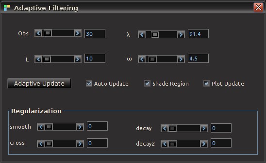Furthermore, since a much shorter span of observations, namely $\tilde{N} << N$ , is being used to construct the new filters, one of the advantages of this filter updating is that it is extremely fast, as well as being effective. As we will show in the next section of this article, all aspects of this dynamic adaptive filtering can be easily controlled, tested, and applied in the MDFA module of iMetrica using a new adaptive filtering control panel. One can control all aspects, from filter length to all the filter parameters in the new updated filter design, and then apply the results to out-of-sample data to compare performance.

Dynamic Adaptive Filtering Interface in iMetrica

The adaptive filtering capabilities in iMetrica are controlled by an interface that allows for adjusting all aspects of the adaptive filter, including number of observations, filter length $L$ , customization controls for timeliness and smoothness, and controls for regularization. The process for controlling and applying dynamic adaptive filtering in iMetrica is accomplished as follows. Firstly, the following two things are required in order to perform dynamic adaptive filtering.

Data. A target time series and (optional) $M$ explanatory series that describe the target series all available on $N$ observations for in-sample filter computation along with a stream of future information flow (i.e. an additional set of, say $\tilde{N}$ , future observations for each of the $M + 1$ series.
An initial set of optimized filter coefficients $b^j_l$ for the signal of the data in-sample.

With these two prerequisites, we are now ready to test different dynamic adaptive filtering strategies. Figure 1 shows the MDFA module interface with time series data of a target series (shown in red) and four explanatory series (not plotted). Using the parameter configuration shown in Figure 1, an initial filter for computing the signal (green plot) that has been optimized in-sample on 300 observations of data and then applied to 30 out-of-sample observations (shown in the blue shaded region). As these final 30 observations of the signal have been produced using 30 out-of-sample observations, we can take note of its out-of-sample performance. Here, the performance of the signal has much room to improve. In this example, we use simulated data (conditionally heteroskedastic data generating process to emulate log-return type data) so that we are able to compare the computed updated signals with a high-order approximation of the target symmetric “perfect” signal (shown in gray in Figure 1).

The original signal (green) built using 300 observations in-sample, and then applied to 30 out-of-sample observations. A high-order approximation to the target symmetric filter is plotted in gray.

Figure 1. The original signal (green) built using 300 observations in-sample, and then applied to 30 out-of-sample observations. A high-order approximation to the target symmetric filter is plotted in gray. The blue shaded region is the region in which we wish to apply dynamic filter updating.

Now suppose we wish to improve performance of the signal in future out-of-sample observations by updating the filter coefficients to produce better smoothness, timeliness, and regularization properties. The first step is to ensure that the “Recompute Filter” option is not on (the checkbox in the Real-Time Filter Design panel. This should have been done already to produce the out-of-sample signal). Then go to the MDFA menu at the top of the software and click on “Adaptive Update”. This will pop open the Adaptive Filtering control panel from which we control everything in the new filter updating coefficients (see Figure 2).

Figure 2. The panel interface for controlling every aspect of updating a filter in real-time.

The controls on the Adaptive Filtering panel are explained as follows:

Obs. Sets the number of the latest observations used in the filter update. This is normally set to however many new observations out-of-sample have been streamed into the time series since the last filter computation. Although one can certainly include observations from the original in-sample period as well by simply setting Obs to a number higher than the number of recent out-of-sample observations. The minimum amount of observations is 10 and the maximum is the total length of the time series.
L. Sets the length of the updating filter. Minimum is 5 and maximum is the number of observations minus 5.
$\lambda$ and $\alpha$ . The customization of timeliness and smoothness parameters for the filter construction. These controls are strictly for the updating filter and independent of the ‘old’ filter.
Adaptive Update. Once content with the settings of the update filter, press this button to compute the new filter and apply to the data. The results of the effects of the new filter will automatically appear in the main plotting canvas, specifically in the region of interest (shaded by blue, see blow).
Auto Update. A check box that, if turned on, will automatically compute the new filter for any changes in the filter parameters and automatically plots the effects of the new filter in the main plotting canvas. This is a nice option to use when visually testing the output of the new filter as one can automatically see effects from any small changes to the parameter setting of the filter. This option also renders the “Adaptive Update” button obsolete.
Shade Region. This check box, when activated, will shade the windowing region at the end of time series in which the updating is taking place. Provides a convenient way to pinpoint the exact region of interest for signal updating. The shaded region will appear in a dark blue shade (as shown in Figures 1, 4,6, and 7).
Plot Updates. Clicking this checkbox on and off will plot the newly updated signal (on position) or the older signal (off position). This is a convenient feature as one is able to easily visually compare the new updated signal with the old signal to test for its effectiveness. If adding out-of-sample data and this feature is turned on, it will also apply the new updated filter coefficients to the new data as it comes in. If in the off position, it will only apply the ‘old’ filter coefficients.
Regularization. All the regularization controls for the updating filter.

To update a signal in real-time, first select the number of observations $\tilde{N}$ and the length of the filter from the Obs and L sliding scrollbars, respectively. This will be the total number of observations used in the adaptive updating. For example, when new dynamics appear in the time series out-of-sample that the original old filter was not able to capture, the filter updating should include this new information. Click the checkbox marked Shade Region to highlight in a dark shade of blue the region in which the updated signal will be computed (this is shown in Figure 1). When the number of observations or length of filter changes, the shaded region reflects these changes and adjusts accordingly. After the region of interest is selected, customization and regularization of the signal can then be applied using the sliding scrollbars. Click the “Auto Update” checkbox to the ‘on’ position to see the effects of the parameterization on the signal computed in the highlighted region automatically. Once content with the filter parameterization, visually comparing the new updated signal with the old signal can be achieved simply by toggling the Plot Updates checkbox. To apply this new filter configuration to out-of-sample data, simply add more out-of-sample data by clicking the out-of-sample slider scrollbar control on the Real-Time Direct Filter control panel (provided that more out-of-sample data is available). This will automatically apply the ‘old’ original filter along with the updated filter on the new incoming out-of-sample data. If not content with the updated signal, simply remove the new out-of-sample data by clicking ‘back’ in the out-of-sample scrollbar, and adjust the parameters to your liking and try again. To continuously update the signal, simply reapply the above process as new out-of-sample data is added. As long as the “Plot Updates” is turned on, the newly adapted signal will always be plotted in the windowed region of interest. See Figures 4-7 to see this process in action.

In this example, as previously mentioned, we computed the original signal in-sample using 300 observations and then applied the filter coefficients to 30 out-of-sample observations (this was produced by checking “Recompute Filter” off). This is plotted in Figure 4, with the blue shaded region highlighting the 30 latest observations, our region of interest. Notice a significant mangling of timeliness and signal amplification in the pass-band of the filter. This is due to bad properties of the filter coefficients. Not enough regularization was applied. Surely enough, the amplitude of the frequency response function in the original filter shows the overshooting in the pass-band (see Figure 5). To improve this signal, we apply an adaptive update by launching the Adaptive Update menu and configuring the new filter. Figure 6 shows the updated filter in the windowed region, where we chose a combination of timeliness and light regularization. There is a significant improvement in the timeliness of the signal. Any changes in the parameterization of the filter space is automatically computed and plotted on the canvas, a huge convenience as we can easily test different parameter configurations to easily identify the signal that satisfies the priorities of the user. In the final plot, Figure 7, we have chosen a configuration with a high amount of regularization to prevent overfitting. Compared with the previous two signals in the region of interest (Figures 4 and 6), we see an even greater mollification of the unwanted amplitude overshooting in the signal, without compromising with a lack of timeliness and smoothness properties. A high-order approximation to the targeted symmetric filter is also plotted in this example for comparison convenience (since the data is simulated, we know the future data, and hence the symmetric filter).

Tune in later this week for an example of Dynamic Adaptive Filtering applied to financial trading.

Applying an update to the signal by allocating the 30 most recent out-of-sample observations and computing a new filter of length 10. The blue shaded region shows the updating region. Here the old filter has been applied to the 30 out-of-sample observations and we notice significant mangling of timeliness and signal amplification in the pass-band of the filter. This is due to bad properties of the filter coefficients. Not enough regularization was applied.

Figure 4. Plot of the signal out-of-sample before applying an update to the signal by allocating the 30 most recent out-of-sample observations and computing a new filter of length 10. The blue shaded region shows the updating region. Here the original old filter constructed in-sample has been applied to the 30 out-of-sample observations and we notice significant mangling of timeliness and signal amplification in the pass-band of the filter. This is due to bad properties of the filter coefficients. Not enough regularization was applied.

Figure 5. The overshooting in the pass-band of the frequency response function multivariate filter. The spikes above one in the pass-band indicate this and will most-likely produce overshooting in the signal out-of-sample.

After filter updating in the final 30 observations. We chose the filter settings in the adaptive filter settings to improve timeliness with a small amount of smoothing. Furthermore, regularization (smooth, decay) were applied to ensure no overfitting. Notice how the properties of the signal are vastly improved (namely timeliness and little to no overshooting).

Figure 6 After filter updating in the final 30 observations. We chose the filter settings in the adaptive filter settings to improve timeliness with a small amount of smoothing. Furthermore, regularization (smooth, decay) was applied to ensure no overfitting. Notice how the properties of the signal are vastly improved (namely timeliness and little to no overshooting).

Not satisfied with the results of our filter update, we can easily adjust the parameters more to find a satisfying configuration. In this example, since the data is simulated, I've computed the symmetric filter to compare my results with the theoretically "perfect" filter. After further adjusting regularization parameters, I end up with this signal shown in the plot. Here, the gray signal is the target symmetric "perfect" signal. The result is a very close fit to the target signal with no overfitting.

Figure 7. Not satisfied with the results of our filter update, we can easily adjust the parameters more to find a satisfying configuration. In this example, since the data is simulated, I’ve computed the symmetric filter to compare my results with the theoretically “perfect” filter. After further adjusting regularization parameters, I end up with this signal shown in the plot. Here, the gray signal is a high-order approximation to the target symmetric “perfect” signal. The result is a very close fit to the target signal with no overfitting.

Hierarchy of Financial Trading Parameters

Posted on November 28, 2012 by Christian Dallas Blakely

Figure 1: A trading signal produced in iMetrica for the daily price index of GOOG (Google) using the log-returns of GOOG and AAPL (Apple) as the explanatory data, The blue-pink line represents the account wealth over time, with a 89 percent return on investment in 16 months time (GOOG recorded a 23 percent return during this time). The green line represents the trading signal built using the MDFA module using the hierarchy of parameters described in this article. The gray line is the log price of GOOG from June 6 2011 to November 16 2012.

In any computational method for constructing binary buy/sell signals for trading financial assets, most certainly a plethora of parameters are involved and must be taken into consideration when computing and testing the signals in-sample for their effectiveness and performance. As traders and trading institutions typically rely on different financial priorities for navigating their positions such as risk/reward priorities, minimizing trading costs/trading frequency, or maximizing return on investment , a robust set of parameters for adjusting and meeting the criteria of any of these financial aims is needed. The parameters need to clearly explain how and why their adjustments will aid in operating the trading signal to their goals in mind. It is my strong belief that any computational paradigm that fails to do so should not be considered a candidate for a transparent, robust, and complete method for trading financial assets.

In this article, we give an in-depth look at the hierarchy of financial trading parameters involved in building financial trading signals using the powerful and versatile real-time multivariate direct filtering approach (MDFA, Wildi 2006,2008,2012), the principle method used in the financial trading interface of iMetrica. Our aim is to clearly identify the characteristics of each parameter involved in constructing trading signals using the MDFA module in iMetrica as well as what effects (if any) the parameter will have on building trading signals and their performance.

With the many different parameters at one’s disposal for computing a signal for virtually any type of financial data and using any financial priority profile, naturally there exists a hierarchy associated with these parameters that all have well-defined mathematical definitions and properties. We propose a categorization of these parameters into three levels according to the clarity on their effect in building robust trading signals. Below are the four main control panels used in the MDFA module for the Financial Trading Interface (shown in Figure 1). They will be referenced throughout the remainder of this article.

Figure 2: The interface for controlling many of the parameters involved in MDFA. Adjusting any of these parameters will automatically compute the new filter and signal output with the new set of parameters and plot the results on the MDFA module plotting canvases.

Figure 3: The main interface for building the target symmetric filter that is used for computing the real-time (nonsymmetric) filter and output signal. Many of the desired risk/reward properties are controlled in this interface. One can control every aspect of the target filter as well as spectral densities used to compute the optimal filter in the frequency domain.

Figure 4: The main interface for constructing Zero-Pole Combination filters, the original paradigm for real-time direct filtering. Here, one can control all the parameters involved in ZPC filtering, visualize the frequency domain characteristics of the filter, and inject the filter into the I-MDFA filter to create “hybrid” filters.

Figure 5: The basic trading regulation parameters currently offered in the Financial Trading Interface. This panel is accessed by using the Financial Trading menu at the top of the software. Here, we have direct control over setting the trading frequency, the trading costs per transaction, and the risk-free rate for computing the Sharpe Ration, all controlled by simply sliding the bars to the desired level. One can also set the option to short sell during the trading period (provided that one is able to do so with the type of financial asset being traded).

The Primary Parameters:

Trading Frequency. As the title entails, the trading frequency governs how often buy/sell signal will occur during the span of the trading horizon. Regardless of minute data, hourly data, or daily data, the trading frequency regulates when trades are signaled and is also a key parameter when considering trading costs. The parameter that controls the trading frequency is defined by the cutoff frequency in the target filter of the MDFA and is regulated in either the Target Filter Design interface (see Figure 3) or, if one is not accustomed to building target filters in MDFA, a simpler parameter is given in the Trading Parameter panel (see Figure 5). In Figure 3, the pass-band and stop-band properties are controlled by any one of the sliding scrollbars. The design of the target filter is plotted in the Filter Design canvas (not shown).

Timeliness of signal. The timeliness of the signal controls the quality of the phase characteristics in the real-time filter that computes the trading signal. Namely, it can control how well turning points (momentum changes) are detected in the financial data while minimizing the phase error in the filter. Bad timeliness properties will lead to a large delay in detecting up/downswings in momentum. Good timeliness properties lead to anticipated detection of momentum in real-time. However, the timeliness must be controlled by smoothness, as too much timeliness leads to the addition of unwanted noise in the trading signal, leading to unnecessary unwanted trades. The timeliness of the filter is governed by the $\lambda$ parameter that controls the phase error in the MDFA optimization. This is done by using the sliding scrollbar marked $\lambda$ in the Real-Time Filter Design in Figure 2. One can also control the timeliness property for ZPC filters using the $\lambda$ scrollbar in the ZPC Filter Design panel (Figure 4).

Smoothness of signal. The smoothness of the signal is related to how well the filter has suppressed the unwanted frequency information in the financial data, resulting in a smoother trading signal that corresponds more directly to the targeted signal and trading frequency. A signal that has been submitted to too much smoothing however will lose any important timeliness advantages, resulting in delayed or no trades at all. The smoothness of the filter can be adjusted through using the $\alpha$ parameter that controls the error in the stop-band between the targeted filter and the computed concurrent filter. 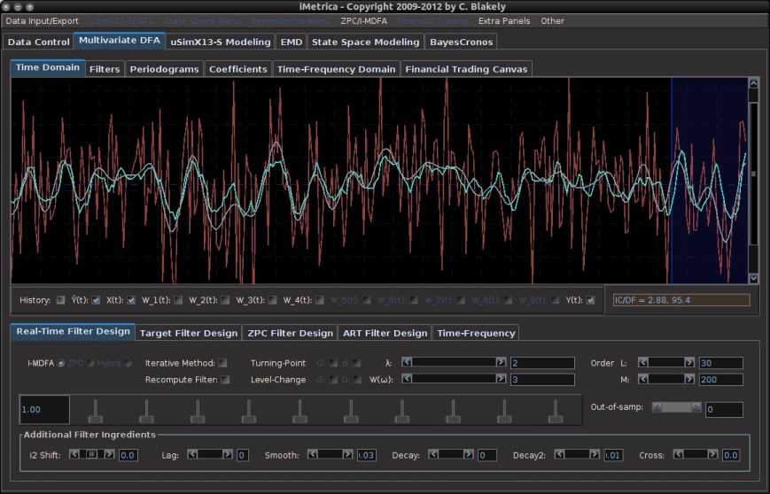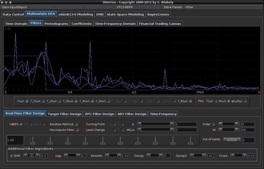The smoothness parameter is found on the Real-Time Filter Design interface in the sliding scrollbar marked $W(\omega)$ (see Figure 2) and in the sliding scrollbar marked $\alpha$ in the ZPC Filter Design panel (see Figure 4).

Quantization of information. In this sense, the quantization of information relates to how much past information is used to construct the trading signal. In MDFA, it is controlled by the length of the filter $L$ and is found on the Real-Time Filter Design interface (see Figure 2). In theory, as the filter length $L$ gets larger. the more past information from the financial time series is used resulting in a better approximation of the targeted filter. However, as the saying goes, there’s no such thing as a free lunch: increasing the filter length adds more degrees of freedom, which then leads to the age-old problem of over-fitting. The result: increased nonsense at the most concurrent observation of the signal and chaos out-of-sample. Fortunately, we can relieve the problem of over-fitting by using regularization (see Secondary Parameters). The length of the filter is controlled in the sliding scrollbar marked Order- $L$ in the Real-Time Filter Design panel (Figure 2).

As you might have suspected, there exists a so-called “uncertainty principle” regarding the timeliness and smoothness of the signal. Namely, one cannot achieve a perfectly timely signal (zero phase error in the filter) while at the same time remaining certain that the timely signal estimate is free of unwanted “noise” (perfectly filtered data in the stop-band of the filter). The greater the timeliness (better phase error), the lesser the smoothness (suppression of unwanted high-frequency noise). A happy combination of these two parameters is always desired, and thankfully there exists in iMetrica an interface to optimize these two parameters to achieve a perfect balance given one’s financial trading priorities. There has been much to say on this real-time direct filter “uncertainty” principle, and the interested reader can seek the gory mathematical details in an original paper by the inventor and good friend and colleague Professor Marc Wildi here.

The Secondary Parameters

Regularization of filters is the act of projecting the filter space into a lower dimensional space,reducing the effective number of degrees of freedom. Recently introduced by Wildi in 2012 (see the Elements paper), regularization has three different members to adjust according to the preferences of the signal extraction problem at hand and the data. The regularization parameters are classified as secondary parameters and are found in the Additional Filter Ingredients section in the lower portion of the Real-Time Filter Design interface (Figure 2). The regularization parameters are described as follows.

Regularization: smoothness. Not to be confused with the smoothness parameter found in the primary list of parameters, this regularization technique serves to project the filter coefficients of the trading signal into an approximation space satisfying a smoothness requirement, namely that the finite differences of the coefficients up to a certain order defined by the smoothness parameter are kept relatively small. This ultimately has the effect that the parameters appear smoother as the smooth parameter increases. Furthermore, as the approximation space becomes more “regularized” according to the requirement that solutions have “smoother” solutions, the effective degrees of freedom decrease and chances of over-fitting will decrease as well. The direct consequences of applying this type of regularization on the signal output are typically quite subtle, and depends clearly on how much smoothness is being applied to the coefficients. Personally, I usually begin with this parameter for my regularization needs to decrease the number of effective degrees of freedom and improve out-of-sample performance.

Regularization: decay. Employing the decay parameter ensures that the coefficients of the filter decay to zero at a certain rate as the lag of the filter increases. In effect, it is another form of information quantization as the trading signal will tend to lessen the importance of past information as the decay increases. This rate is governed by two decay parameter and higher the value, the faster the values decrease to zero. The first decay parameter adjusts the strength of the decay. The second parameter adjusts for how fast the coefficients decay to zero. Usually, just a slight touch on the strength of the decay and then adjusting for the speed of the decay is the order in which to proceed for these parameters. As with the smoothing regularization, the number of effective degrees of freedom will (in most cases) decreases as the decay parameter decreases, which is a good thing (in most cases).

Regularization: cross correlation. Used for building trading signals with multivariate data only, this regularization effect groups the latitudinal structure of the multivariate time series more closely, resulting in more weighted estimate of the target filter using the target data frequency information. As the cross regularization parameter increases, the filter coefficients for each time series tend to converge towards each other. It should typically be used in a last effort to control for over-fitting and should only be used if the financial time series data is on the same scale and all highly correlated.

The Tertiary Parameters

Phase-delay customization. The phase-delay of the filter at frequency zero, defined by the instantaneous rate of change of a filter’s phase at frequency zero, characterizes important information related to the timeliness of the filter. One can directly ensure that the phase delay of the filter at frequency zero is zero by adding constraints to the filter coefficients at computation time. This is done by setting the clicking the $i2$ option in the Real-Time Filter Design interface. To go further, one can even set the phase delay to an fixed value other than zero using the $i2$ scrollbar in the Additional Filter Ingredients box. Setting this value to a certain value (between -20 and 20 in the scrollbar) ensures that the phase delay at zero of the filter reacts as anticipated. It’s use and benefit is still under investigation. In any case, one can seamlessly test how this constraint affects the trading signal output in their own trading strategies directly by visualizing its performance in-sample using the Financial Trading canvas.

Differencing weight. This option, found in the Real-Time Filter Design interface as the checkbox labeled “d” (Figure 2), multiplies the frequency information (periodogram or discrete Fourier transform (DFT)) of the financial data by the weighting function $f(\omega) = 1/(1 - \exp(i \omega)), \omega \in (0,\pi)$ , which is the reciprocal of the differencing operator in the frequency domain. Since the Financial Trading platform in iMetrica strictly uses log-return financial time series to build trading signals, the use of this weighting function is in a sense a frequency-based “de-differencing” of the differenced data. In many cases, using the differencing weight provides better timeliness properties for the filter and thus the trading signal.

In addition to these three levels of parameters used in building real-time trading signals, there is a collection of more exotic “parameterization” strategies that exist in the iMetica MDFA module for fine tuning and constructing boosting trading performance. However, these strategies require more time to develop, a bit of experimentation, and a keen eye for filtering. We will develop more information and tutorials about these advanced filtering techniques for constructing effective trading signals in iMetrica in future articles on this blog coming soon. For now, we just summarize their main ideas.

Advanced Filtering Parameters

Hybrid filtering. In hybrid filtering, the goal is to filter a target signal additionally by injecting it with another filter of a different type that was constructed using the same data, but different paradigm or set of parameters. One method of hybrid filtering that is readily available in the MDFA module entails constructing Zero-Pole Combination filters using the ZPC Filter Design interface (Figure 4) and injecting the filter into the filter constructed in the Real-Time Filter Design interface (Figure 2) (see Wildi ZPC for more information). The combination (or hybrid) filter can then be accessed using one of the check box buttons in the filter interface and then adjusted using all the various levels of parameters above, and then used in the financial trading interface. The effect of this hybrid construction is to essentially improve either the smoothness or timeliness of any computed trading signal, while at the same time not succumbing to the nasty side-effects of over-fitting.

Forecasting and Smoothing signals. Smoothing signals in time series, as its name implies, involves obtaining a smoother estimate of certain signal in the past. Since the real-time estimate of a signal value in the past involves using more recent values, the signal estimation becomes more symmetrical as past and future values at a point in the past are used to estimate the value of the signal. For example, if today is after market hours on Friday, we can obtain a better estimate of the targeted signal for Wednesday since we have information from Thursday and Friday. In the opposite manner, forecasting involves projecting a signal into the future. However, since the estimate becomes even more “anti-symmetric”, the estimate becomes more polluted with noise. How these smoothed and forecasted signals can be used for constructing buy/sell trading signals in real-time is still purely experimental. With iMetrica, building and testing strategies that improve trading performance using either smoothed and forecasted signals (or both), is available.To produce either a smoothed or forecasted signal, there is a lag scrollbar available in the Real-Time Filter Design interface under Additional Filter Ingredients that enables one to compute either a smooth or forecasted signal. Setting the lag value $k$ in the scrollbar to any integer between -10 and 10 and the signal with the set lag applied is automatically computed. For negative lag values $k$ , the method produces a $k$ step-ahead forecast estimate of the signal. For positive values, the method produces a smoothed signal with a delay of $k$ observations.

Customized spectral weighting functions. In the spirit of customizing a trading signal to fit one’s priorities in financial trading, one also has the option of customizing the spectral density estimate of the data generating process to any design one wishes. In the computation of the real-time filter, the periodogram (or DFTs in multivariate case) is used as the default estimate of the spectral density weighting function. This spectral density weighting function in theory is supposed to serve as the spectrum of the underlying data generating process (DGP). However, since we have no possible idea about the underlying DGP of the price movement of publicly traded financial assets (other than it’s supposed to be pretty darn close to a random walk according to the Efficient Market Hypothesis), the periodogram is the best thing to an unbiased estimate a mortal human can get and is the default option in the MDFA module of iMetrica. However, customization of this weighting function is certainly possible through the use of the Target Filter Design interface. Not only can one design their target filter for the approximation of the concurrent filter, but the spectral density weighting function of the DGP can also be customized using some of the available options readily available in the interface. We will discuss these features in a soon-to-come discussion and tutorial on advanced real-time filtering methods.

Adaptive filtering. As perhaps the most advanced feature of the MDFA module, adaptive filtering is an elegant way to achieve building smarter filters based on previous filter realizations. With the goal of adaptive filtering being to improve certain properties of the output signal at each iteration without compensating with over-fitting, the adaptive process is of course highly nonlinear. In short, adaptive MDFA filtering is an iterative process in which a one begins with a desired filter, computes the output signal, and then uses the output signal as explanatory data in the next filtering round. At each iteration step, one has the freedom to change any properties of the filter that they desire, whether it be customization, regularization, adding negative lags, adding filter coefficient constraints, applying a ZPC filter, or even changing the pass-band in the target filter. The hope is to improve on certain properties of filter at each stage of the iterative process. An in-depth look at adaptive filtering and how to easily produce an adaptive filter using iMetrica is soon to come later this week.

iMetrica: Economic and Financial Data Control

Posted on November 14, 2012 by Christian Dallas Blakely

The iMetrica software is endowed with a rich and detailed, yet quite easy-to-use module for uploading, downloading, exporting, editing, combining, transforming, building, simulating, and analyzing time series data. It contains just about anything you’d want to have in an economic or financial time series data control interface while using only simple mouse point-and-click or drag interactions to navigate or download data from the internet. Since the most important aspect of time series analysis is, well, the time series data itself, we created a dedicated data control module to handle the majority of the time series data loading and editing work, before it is exported to any one of the five iMetrica computational modules or financial trading module.

Data Control Interface

We begin this iMetrica blog entry by first giving an overview of the basic components featured in the Data Control module. Figures 1 and 2 show the interface and all the major components labeled. Here, a collection of simulated time series are being plotted together.

Figure 1. The major components of the data control module.

Figure 2. The major components of the data control module, showing the target series editor.

Main plotting canvas. This is where the time series data is plotted. Up to 10 different time series can be loaded into the data control at a time, and all of them can be plotted using the plot control in panel 2. When all the data is plotted together, to highlight a particular series, go to the main Data Control menu in the top left corner and place the mouse on any one the series names, the respective series will then be highlighted.
Plot control panel. The time series that are uploaded into the module can be viewed by toggling their respective check box inside the plot control panel. This is helpful when different time series are scaled different and/or have different means. One can also log-transform the data, rescale the data to have unit standard deviations, or compare data using cross-correlations. Note that the log and rescale check box actions will only apply to the data that is currently being plotted. Furthermore, to plot the cross-correlations, only two time series can be chosen at a time. When one time series is chosen, the auto-correlation plot is drawn. Here, the “Target $X(t)$ indicates a weighted aggregation of the data. To edit this, use the “Target Series” in 3. To delete all of the data stored in the data control module, simply press the “Delete” button. Careful, there’s no going back once deleted.
Simulated and Target Series Panels. The simulated time series data interfaces to simulate a multitude of different time series. Simulating time series can be helpful when wanting to either learn, practice, or explore the different modules and capabilites of iMetrica, learn more about time series analysis, or learn about the dynamics of time series modules. The different types of models include (S)ARIMA models, GARCH models, correlated cycle models, trend models, multivariate factor stochastic volatility models, and HEAVY models. From simulating data and toggling the parameters, one can visualize instantly the effects of the each parameter on the simulated data. The data can then be exported to any of the modules for practicing and honing one’s skills in hybrid modeling, signal extraction, and forecasting. Each model has a “parameter” button (see 4) that controls the dimensions, innovation distributions, or parameter values. When changes are made, the simulated series is recomputed automatically and replotted on their respective plotting canvas (see 4).
Simulated Data Control. Once the parameters have been selected, and a desired simulated series has been achieved to one’s liking, it can be added to the main data control plotting canvas by clicking the “Add” button. The new simulated series is now ready to be exported to any of the modules. One can also change the random seed that controls the “burn-in” of the innovation sequence (random effects that govern the initialization and trajectory of the data). In some of the models, one can “integrate” the data to render stationary data nonstationary.
Parameter Controls. Once the “Parameters” button has been clicked, an additional panel will pop up where controls for all the model’s parameters can be toggled. Once any parameter has been changed using the sliders, scrollbars, or combo boxes, the simulated data is automatically recomputed and plotted, making it a great tool to understand time series model dynamics.
Target Series Construction. The target series is used to construct a univariate time series that is a weighted sum of one or more time series (given by the $X_i(t)$ for $i=1,\ldots,10$ series). In modules that only deal with univariate time series data (the uSimX13, EMD, and State Space Modeling), the constructed target series is the series that gets exported for analysis. For the MDFA module, this is the series that is being filtered for constructing a signal, with the other time series acting as the explanatory time series. In the BayesCronos module, this target series is ignored and only the supporting time series data $X_i(t)$ are used. In these up and down slider controls, one can adjust for the weight associated with that specific series, and the aggregate target series will be automatically recomputed as it is adjusted.
Series Checkboxes. To ignore the series entirely in the computation of the target series, simply click the check box “off” in the associated “computed in target” check box. This will eliminate it from the target sum. In the case one is constructing data for the MDFA module, one has the option of utilizing a series in the target series, but not using it as an explaining time series variable, and vice-versa.

Loading Data from Files

Within this main data control hub, one can import univariate or multivariate time series data from a multitude of file formats, as well as download financial time series data directly from Yahoo! finance or another source such as Reuters for higher-frequency financial data. To load data from a file, simply click on the “Data Input/Export” menu when in the Data Control module and select one of the “Load” data options. The “Load Data” option pop up a “file select” panel and from there, the data file can be selected. The format of the data in this “Load Data” case is simple: a single column of data for each series. If more than one series is present, the data column must be separated by a space. In the “Load CSV” data, this assumes the file is stored in a CSV format. See Figure 3 for the menu options of the Data Control module.

Figure 3. Showing the different options for importing data into the data control module.

Downloading Financial Data

The other option for loading data into the module is through the “Load Market Data” interface. Rather than loading data from a file that is sitting in your directory, you also conveniently have the option to download data directly from the internet or financial time series database, such as Reuters. As a fast and easy way to download financial data into iMetrica, when the “Load Market Data” is selected, a pop-up panel interface will surface that gives access to controlling the download of financial market data. This is shown in Figure 4. The options on this interface are described below.

Figure 4. The “Load Market Data” interface to download market data directly from Yahoo!. Here the daily log-returns and volume of Google (GOOG) and Apple (AAPL) are being downloaded.

Symbols(s) – In this text box, type the market ticker symbol of the desired financial series in all CAPS. Each ticker symbol must be seperated only by one space and nothing else. Up to 10 ticker symbols can be entered.
Start Date – This indicates the year, month, and day from which the financial time series begins. This date must obviously be in the past. If the day falls on a non-traded day such as a weekend or holiday, the nearest date after that date will be chosen. The time series will then be loaded to the most recent date available for that asset.
Hours – This indicates the time period in which the frequency of the data is selected. In most cases, this should simply be set to “US Market Hours”.
Frequency – The frequency of the data. The options are Second, Minute, 3,5,10,15,30-Minute, Hourly, Daily, Weekly, Monthly.
New Data Set – Deletes all the data already stored in the data control module and uploads as new data.
Log Returns – Download the data in log-return format. This is usually the case when using the data to build financial trading strategies using the MDFA module. However, in addition to the log-return data, it will also download the log-transformed raw time series data of the first asset in the Symbols(s) box. This is generally used for gauging financial trading accounts in the financial trading interface of iMetrica. When Financial Trading is turned on in the data control menu this is automatically set on.
Volume Data – In addition to the asset time series data, the volume (of trades) data associated for the given frequency will also be downloaded for each market ticker symbol given in Symbols(s).
Yahoo! Source – The financial data will be downloaded from Yahoo! finance (thus you need an internet connection). If this box is not checked, then the downloader will assume a Reuters financial database (but of course for this you need an account with Reuters).

Once the settings are made in the interface, click “Download Market Data”. If no errors are present in the settings, then all the data should be automatically available in the plot canvas after a few seconds of downloading time. Figure 5 gives the results of the data download from the example in Figure 4. Here, the daily log-returns of Google (GOOG) and Apple (AAPL) along with their daily volumes from 6-4-2011 to today (11-14-2012) have been downloaded into the data control module and ready for use. Notice the scaling of the volume data (final two series) have been adjusted using the simple slider bars in the “Target Series” panel to more-or-less fit the scale of the log-return data.

Figure 5. The daily log-returns of Google (GOOG) and Apple (AAPL) along with their respective volumes loaded into the data control module and plotted on the canvas. The data was uploaded by using the “Load Market Data” interface panel.

If there were errors, then no data will be uploaded to the canvas and you have to try again. Common errors are either no internet connection, the symbols are either incorrect or not in CAPS, or the starting date is bogus. Once the data is available to be plotted, simply click the check boxes associated with each plot. edit, scale, export, analyse, compute, and/or trade away!

More options for downloading data will constantly be added to the iMetrica software. Check back to the blog regularly for more updates and additions as they come. Of course, suggestions are always welcome.

iMetrica and Hybridometrics: Introduction

Posted on October 24, 2012 by Christian Dallas Blakely

The high-frequency Financial Trading interface of iMetrica. Easily construct in-sample trading strategies with an array of optimizers unique to iMetrica and then employ the strategies out-of-sample to test and fine-tune the trading performance.

This blog serves as an introduction and tutorial to Hybridometrics using iMetrica. Hybridometrics is a term used to express the analysis, modeling, signal extraction, and forecasting of univariate and multivariate financial and economic time series data using a combination of model-based and non-model-based methodologies. Ideal combinations of computational paradigms and methodologies used in hybridometrics include, but are not limited to, traditional stochastic models such as (S)ARIMA models, GARCH models, and multivariate stochastic volatiluty models combined with empirical mode decomposition techniques and the multivariate direct filter approach (MDFA). The goal of hybridometric modeling is to obtain signal extractions and forecasts, for official use or government use, all the way to building high-frequency financial trading strategies, that perform better than using only model or non-model based methods alone. In other words, hybridometrics seeks to extract the advantages of different paradigms combined to outperform traditional approaches to time series modeling. The iMetrica software package offers the most versatile and computationally efficient portal to this newly proposed time series modeling paradigm, all while remaining surprisingly easy to use.

The iMetrica software package is a unique system of econometric and financial trading tools that focuses on speed, user interaction, visualization tools, and point-and-click simplicity in building models for time series data of all types. Written entirely in GNU C and Fortran with a rich interactive interface written in Java, the iMetrica software offers an abundance of econometric tools for signal extraction and forecasting in multivariate time series that are both easily accessible with the click of a mouse button and fast with results computed and plotted instantaneously without the need for creating output data files or calling exterior plotting devices.

One powerful feature that is unique to the iMetrica software is the innate capability of easily combining both model-based and non-model based methodologies for designing data forecasts, signal extraction filters, or high-frequency financial trading strategies. Furthermore, the strategies can be computed and tested both in-sample and out-of-sample using an easy to use built-in data partitioner that effectively partitions the data into an in-sample storage where models and filters are computed and then an out-of-sample storage where new data is applied to the in-sample strategy to test for robustness, over-fitting, and many other desired properties. This gives the user complete liberty in creating a fast and efficient test-bed for implementing signal extractions, forecasting regimes, or financial trading strategies.

The iMetrica software environment includes five interacting time series analysis modules for building hybrid forecasts, signal extractions, and trading strategies.

uSimX13 – A computational environment for univariate seasonal auto-regressive integrated moving-average (SARIMA) modeling and simulation using X-13ARIMA-SEATS. Features an interactive approach to modeling seasonal economic time series with SARIMA models and automatic outlier detection, trading day, and holiday regressor effects. Also includes a suite of model comparison tools using both modern and goodness-of-fit signal extraction diagnostics.
BayesCronos – An interactive time series module for signal extraction and forecasting of multivariate economic and financial time series focusing on Bayesian computation and simulation. This module includes a multitude of models including ARIMA, GARCH, EGARCH, Stochastic Volatility, Multivariate Factor Stochastic Volatility, Dynamic Factor, and Multivariate High-Frequency-Based Volatility (HEAVY), with more models continuously being added. For most of the models featured, one can compute the Bayesian and/or the Quasi-Maximum-Likelihood estimated model fits using either a Metropolis-Hastings Monte Carlo Markov Chain approach (Bayesian) or a QMLE formulation for computing the model parameters estimates. Using a convenient model selection panel interface, complete access to model-type, model parameter dimensions, prior distribution parameters is seamlessly available. In the case of Bayesian estimation, one has complete control over the prior distributions of the model parameters and offers interactive visualization of the Monte Carlo Markov Chain parameter samples. For each model, up to 10 sample 36-steps ahead forecasts can be produced and visualized instantaneously along with other important model features such as model residuals, computed volatility, forecasted volatility, factor models, and more. The results can then be easily exported to other modules in iMetrica for additional filtering and/or modeling.
MDFA – An interactive interface to the most comprehensive multivariate real-time direct filter analysis and computation environment in the world. Build real-time filters using both I-MDFA and Zero-Pole Combination (ZPC) filter constructions. The module includes interactive access to timeliness, smoothing, and accuracy controls for filter customization along with parameters for filter regularization to control overfitting. More advanced features include an interface for building adaptive filters, and many controls for filter optimization, customization, data forecasting, and target filter construction.
State Space Modeling – A module for building observed component ARIMA and regression models for univariate economic time series. Similar to the uSimX13 module, the State Space Modeling environment focuses on modeling and forecasting economic time series data, but with much more generality than SARIMA models. An aggregation of observed stochastic components in the form of ARIMA models are stipulated for the time series data (for example trend + seasonal + irregular) and then regression components to model outliers, holiday, and trading day effects are added to the stochastic components giving ultimate flexibility in model building. The module uses regCMPNT, a suite of Fortran code written at the US Census Bureau, for the maximum likelihood and Kalman filter computational routines.
EMD – The EMD module offers a time-frequency decomposition environment for the time-frequency analysis of time series data. The module offers both the original empirical mode decomposition technique of Huan et al. using cubic splines, along with an adaptive approach using reproducing kernels and direct-filtering. This empirical decomposition technique decomposes nonlinear and nonstationary time series into amplitude modulated and frequency modulated (AM-FM) components and then computes the intrinsic phase and instantaneous frequency components from the FM components. All plots of the components as well as the time-frequency heat maps are generated instantaneously.

Along with these modules, there is also a data control module that handles all aspects of time series data input and export. Within this main data control hub, one can import multivariate time series data from a multitude of file formats, as well as download financial time series data directly from Yahoo! finance or another source such as Reuters for higher-frequency financial data. Once the data is loaded, the data can be normalized, scaled, demeaned, and/or log-transformed with a simple slider and button controls, with the effects being plotted on the graphic canvas instantaneously.

Another great feature of the iMetrica software is the ability to learn more about time series modeling through the using of data simulators. The data control module includes an array of data simulating panels for simulating data from a multitude of both univariate and multivariate time series models. With access to control the number of observations, the random seed for the innovation process, the innovation process distribution, and the model parameters, simulated data can be constructed for any type of economic or financial time time series imaginable. The different types of models include (S)ARIMA models, GARCH models, correlated cycle models, trend models, multivariate factor stochastic volatility models, and HEAVY models. From simulating data and toggling the parameters, one can visualize instantly the effects of the each parameter on the simulated data. The data can then be exported to any of the modules for practicing and honing one’s skills in hybrid modeling, signal extraction, and forecasting.

Keep visiting this blog frequently for continuous updates, tutorials, and proposals in the field of econometrics, signal extraction, forecasting, and high-frequency financial trading. using hybridometrics and iMetrica.

Hybrid Signal Extraction, Machine Learning, and Algorithmic Financial Trading

Combining Computational Methodologies for Real-Time Learning and Signal Extraction

Tag Archives: financial trading