The multivariate direct filter approach (MDFA) is a generic real-time signal extraction and forecasting framework endowed with a richly parameterized interface allowing for adaptive and fully-regularized data analysis in large multivariate time series. The methodology is based primarily in the frequency domain, where all the optimization criteria is defined, from regularization, to forecasting, to filter constraints. For an in-depth tutorial on the mathematical formation, the reader is invited to check out any of the many publications or tutorials on the subject from blog.zhaw.ch.
This MDFA-Toolkit (clone here) provides a fast, modularized, and adaptive framework in JAVA for doing such real-time signal extraction for a variety of applications. Furthermore, we have developed several components to the package featuring streaming time series data analysis tools not known to be available anywhere else. Such new features include:
- A fractional differencing optimization tool for transforming nonstationary time-series into stationary time series while preserving memory (inspired by Marcos Lopez de Prado’s recent book on Advances in Financial Machine Learning, Wiley 2018).
- Easy to use interface to four different signal generation outputs:
Univariate series -> univariate signal
Univariate series -> multivariate signal
Multivariate series -> univariate signal
Multivariate series -> multivariate signal - Generalization of optimization criterion for the signal extraction. One can use a periodogram, or a model-based spectral density of the data, or anything in between.
- Real-time adaptive parameterization control – make slight adjustments to the filter process parameterization effortlessly
- Build a filtering process from simpler user-defined filters, applying customization and reducing degrees of freedom.
This package also provides an API to three other real-time data analysis frameworks that are now or soon available
- iMetricaFX – An app written entirely in JavaFX for doing real-time time series data analysis with MDFA
- MDFA-DeepLearning – A new recurrent neural network methodology for learning in large noisy time series
- MDFA-Tradengineer – An automated algorithmic trading platform combining MDFA-Toolkit, MDFA-DeepLearning, and Esper – a library for complex event processing (CEP) and streaming analytics
To start the most basic signal extraction process using MDFA-Toolkit, three things need to be defined.
- The data streaming process which determines from where and what kind of data will be streamed
- A transformation of the data, which includes any logarithmic transform, normalization, and/or (fractional) differencing
- A signal extraction definition which is defined by the MDFA parameterization
Data streaming
In the current version, time series data is providing by a streaming CSVReader, where the time series index is given by a String DateTime stamp is the first column, and the value(s) are given in the following columns. For multivariate data, two options are available for streaming data. 1) A multiple column .csv file, with each value of the time series in a separate column 2) or in multiple referenced single column time-stamped .csv files. In this case, the time series DateTime stamps will be checked to see if in agreement. If not, an exception will be thrown. More sophisticated multivariate time series data streamers which account for missing values will soon be available.
Transforming the data
Depending on the type of time series data and the application or objectives of the real time signal extraction process, transforming the data in real-time might be an attractive feature. The transformation of the data can include (but not limited to) several different things
- A Box-Cox transform, one of the more common transformations in financial and other non-stationary time series.
- (fractional)-differencing, defined by a value d in [0,1]. When d=1, standard first-order differencing is applied.
- For stationary series, standard mean-variance normalization or a more exotic GARCH normalization which attempts to model the underlying volatility is also available.
Signal extraction definition
Once the data streaming and transformation procedures have been defined, the signal extraction parameters can then be set in a univariate or multivariate setting. (Multiple signals can be constructed as well, so that the output is a multivariate signal. A signal extraction process can be defined by defining and MDFABase object (or an array of MDFABase objects in the mulivariate signal case). The parameters that are defined are as follows:
- Filter length: the length L in number of lags of the resulting filter
- Low-pass/band-pass frequency cutoffs: which frequency range is to be filtered from the time-series data
- In-sample data length: how much historical data need to construct the MDFA filter
- Customization: α (smoothness) and λ (timeliness) focuses on emphasizing smoothness of the filter by mollifying high-frequency noise and optimizing timeliness of filter by emphasizing error optimization in phase delay in frequency domain
- Regularization parameters: controls the decay rate and strength, smoothness of the (multivariate) filter coefficients, and cross-series similarity in the multivariate case
- Lag: controls the forecasting (negative values) or smoothing (positive values)
- Filter constraints i1 and i2: Constrains the filter coefficients to sum to one (i1) and/or the dot product with (0,1…, L) is equal to the phase shift, where L is the filter length.
- Phase-shift: the derivative of the frequency response function at the zero frequency.
All these parameters are controlled in an MDFABase object, which holds all the information associated with the filtering process. It includes it’s own interface which ensures the MDFA filter coefficients are updated automatically anytime the user changes a parameter in real-time.
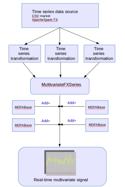
Figure 1: Overview of the main module components of MDFA-Toolkit and how they are connected
As shown in Figure 1, the main components that need to be defined in order to define a signal extraction process in MDFA-Toolkit. The signal extraction process begins with a handle on the data streaming process, which in this article we will demonstrate using a simple CSV market file reader that is included in the package. The CSV file should contain the raw time series data, and ideally a time (or date) stamp column. In the case there is no time stamp column, such a stamp will simply be made up for each value.
Once the data stream has been defined, these are then passed into a time series transformation process, which handles automatically all the data transformations which new data is streamed. As we’ll see, the TargetSeries object defines such transformations and all streaming data is passed added directly to the TargetSeries object. A MultivariateFXSeries is then initiated with references to each TargetSeries objects. The MDFABase objects contain the MDFA parameters and are added to the MultivariateFXSeries to produce the final signal extraction output.
To demonstrate these components and how they come together, we illustrate the package with a simple example where we wish to extract three independent signals from AAPL daily open prices from the past 5 years. We also do this in a multivariate setting, to see how all the components interact, yielding a multivariate series -> multivariate signal.
//Define three data source files, the first one will be the target series
String[] dataFiles = new String[]{"AAPL.daily.csv", "QQQ.daily.csv", "GOOG.daily.csv"};
//Create a CSV market feed, where Index is the Date column and Open is the data
CsvFeed marketFeed = new CsvFeed(dataFiles, "Index", "Open");
/* Create three independent signal extraction definitions using MDFABase:
One lowpass filter with cutoff PI/20 and two bandpass filters
*/
MDFABase[] anyMDFAs = new MDFABase[3];
anyMDFAs[0] = (new MDFABase()).setLowpassCutoff(Math.PI/20.0)
.setI1(1)
.setHybridForecast(.01)
.setSmooth(.3)
.setDecayStart(.1)
.setDecayStrength(.2)
.setLag(-2.0)
.setLambda(2.0)
.setAlpha(2.0)
.setSeriesLength(400);
anyMDFAs[1] = (new MDFABase()).setLowpassCutoff(Math.PI/10.0)
.setBandPassCutoff(Math.PI/15.0)
.setSmooth(.1)
.setSeriesLength(400);
anyMDFAs[2] = (new MDFABase()).setLowpassCutoff(Math.PI/5.0)
.setBandPassCutoff(Math.PI/10.0)
.setSmooth(.1)
.setSeriesLength(400);
/*
Instantiate a multivariate series, with the MDFABase definitions,
and the Date format of the CSV market feed
*/
MultivariateFXSeries fxSeries = new MultivariateFXSeries(anyMDFAs, "yyyy-MM-dd");
/*
Now add the three series, each one a TargetSeries representing the series
we will receive from the csv market feed. The TargetSeries
defines the data transformation. Here we use differencing order with
log-transform applied
*/
fxSeries.addSeries(new TargetSeries(1.0, true, "AAPL"));
fxSeries.addSeries(new TargetSeries(1.0, true, "QQQ"));
fxSeries.addSeries(new TargetSeries(1.0, true, "GOOG"));
/*
Now start filling the fxSeries will data, we will start with
600 of the first observations from the market feed
*/
for(int i = 0; i < 600; i++) {
TimeSeriesEntry observation = marketFeed.getNextMultivariateObservation();
fxSeries.addValue(observation.getDateTime(), observation.getValue());
}
//Now compute the filter coefficients with the current data
fxSeries.computeAllFilterCoefficients();
//You can also chop off some of the data, he we chop off 70 observations
fxSeries.chopFirstObservations(70);
//Plot the data so far
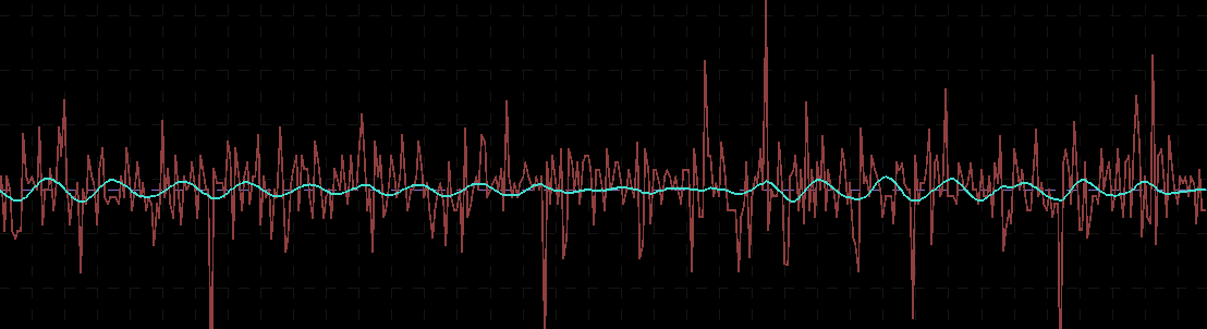
fxSeries.plotSignals("Original");
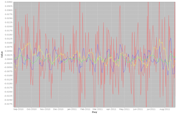
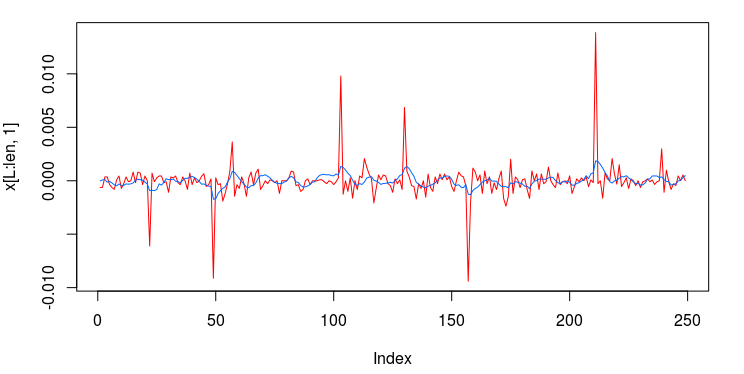
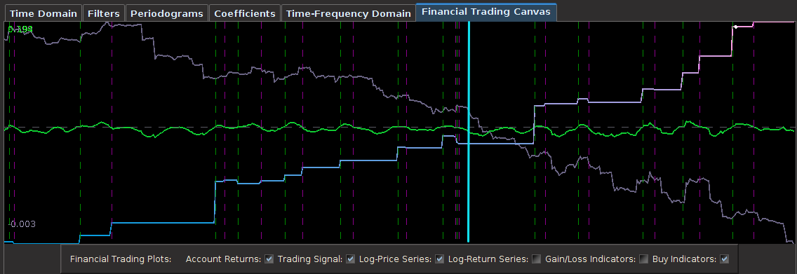
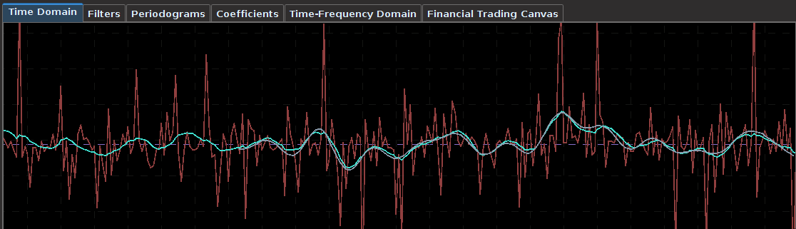
Figure 2: Output of the three signals on the target series (red) AAPL
In the first line, we reference three data sources (AAPL daily open, GOOG daily open, and SPY daily open), where all signals are constructed from the target signal which is by default, the first series referenced in the data market feed. The second two series act as explanatory series. The filter coeffcients are computed using the latest 400 observations, since in this example 400 was used as the insample setSeriesLength, value for all signals. As a side note, different insample values can be used for each signal, which allows one to study the affects of insample data sizes on signal output quality. Figure 2 shows the resulting insample signals created from the latest 400 observations.
We now add 600 more observations out-of-sample, chop off the first 400, and then see how one can change a couple of parameters on the first signal (first MDFABase object).
for(int i = 0; i < 600; i++) {
TimeSeriesEntry observation = marketFeed.getNextMultivariateObservation();
fxSeries.addValue(observation.getDateTime(), observation.getValue());
}
fxSeries.chopFirstObservations(400);
fxSeries.plotSignals("New 400");
/* Now change the lowpass cutoff to PI/6
and the lag to -3.0 in the first signal (index 0) */
fxSeries.getMDFAFactory(0).setLowpassCutoff(Math.PI/6.0);
fxSeries.getMDFAFactory(0).setLag(-3.0);
/* Recompute the filter coefficients with new parameters */
fxSeries.computeFilterCoefficients(0);
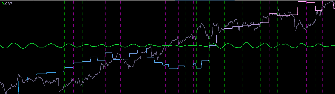
fxSeries.plotSignals("Changed first signal");
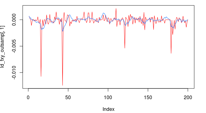
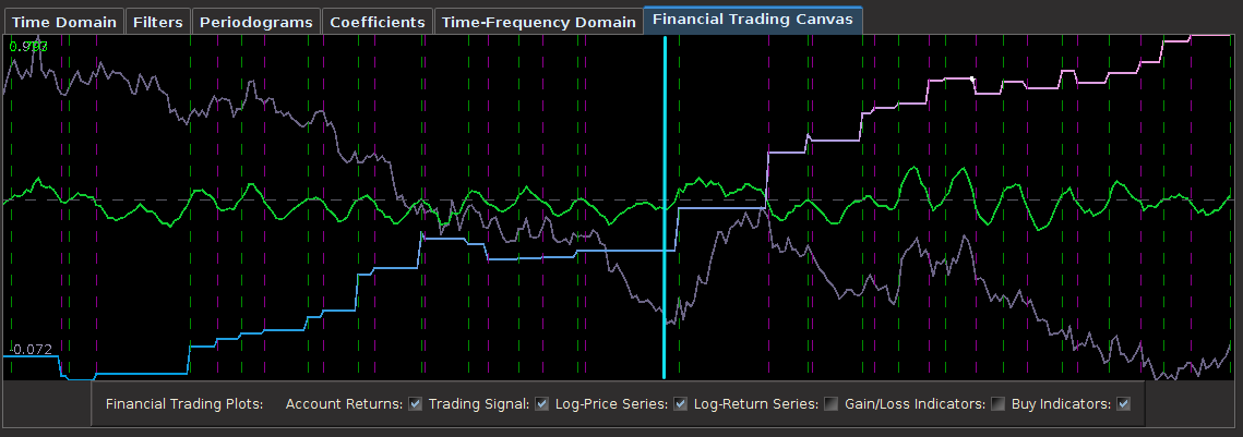
Figure 3: After adding 600 new observations out-of-sample signal values
After adding the 600 values out-of-sample and plotting, we then proceed to change the lowpass cutoff of the first signal to PI/6, and the lag to -3.0 (forecasting three steps ahead). This is done by accessing the MDFAFactory and getting handle on first signal (index 0), and setting the new parameters. The filter coefficients are then recomputed on the newest 400 values (but now all signal values are insample).
In the MDFA-Toolkit, plotting is done using JFreeChart, however iMetricaFX provides an app for building signal extraction pipelines with this toolkit providing the backend where all the automated plotting, analysis, and graphics are handled in JavaFX, creating a much more interactive signal extraction environment. Many more features to the MDFA-Toolkit are being constantly added, especially in regard to features boosting applications in Machine Learning, such as we will see in the next upcoming article.
Big Data analytics in time series
We also implement in MDFA-Toolkit an interface to Apache Spark-TS, which provides a Spark RDD for Time series objects, geared towards high dimension multivariate time series. Large-scale time-series data shows up across a variety of domains. Distributed as the spark-ts package, a library developed by Cloudera’s Data Science team essentially enables analysis of data sets comprising millions of time series, each with millions of measurements. The Spark-TS package runs atop Apache Spark. A tutorial on creating an Apache Spark-TS connection with MDFA-Toolkit is currently being developed.


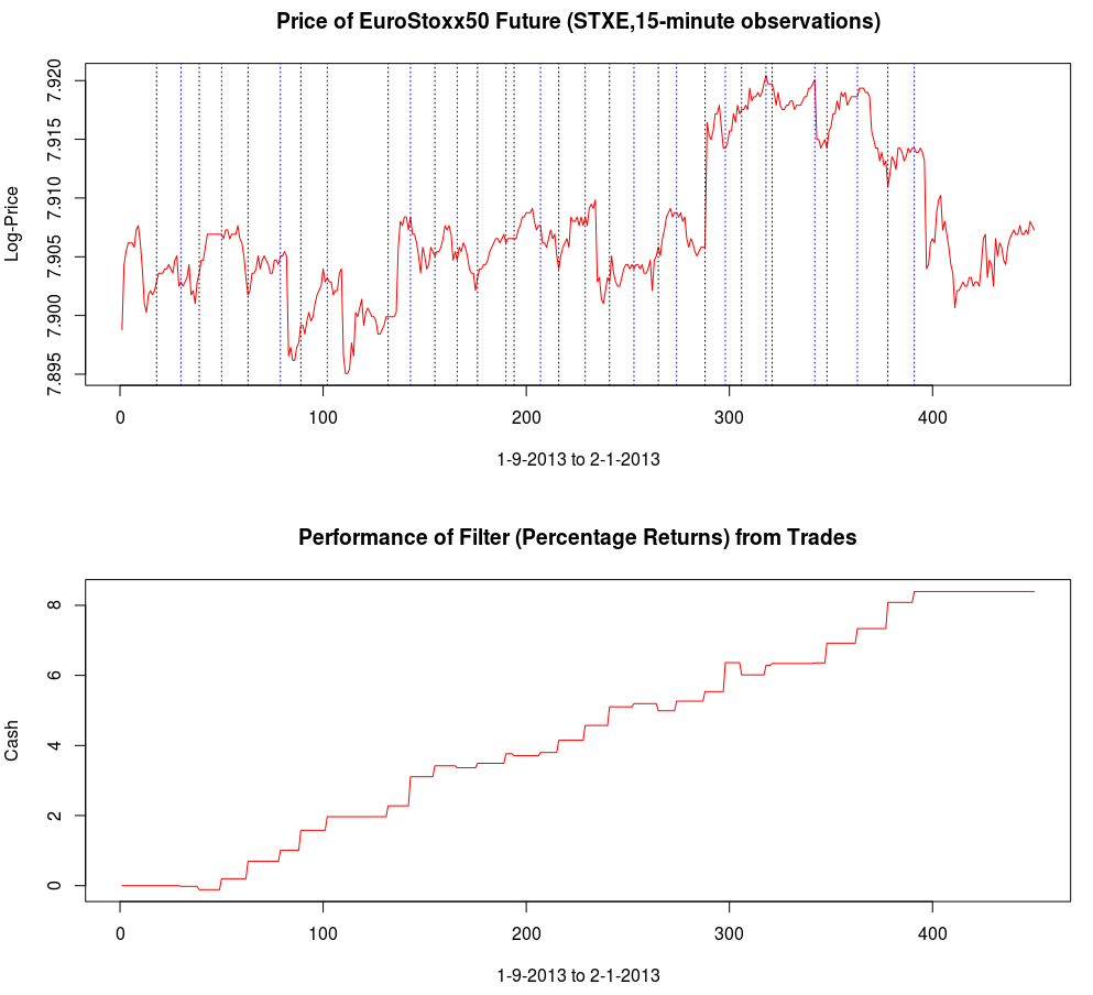
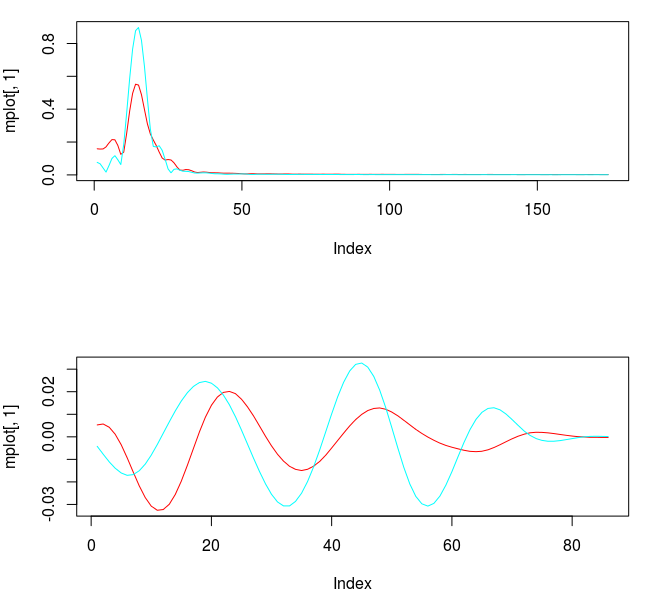
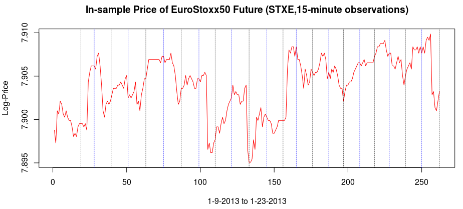
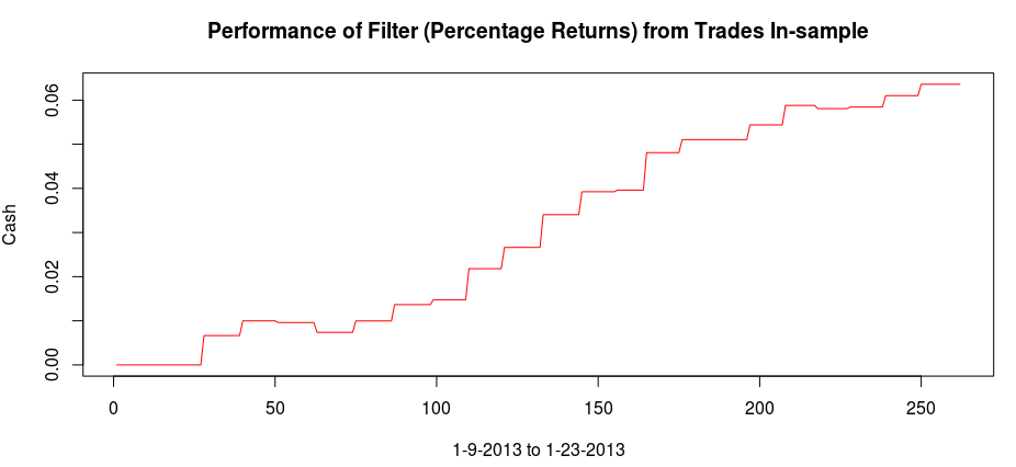
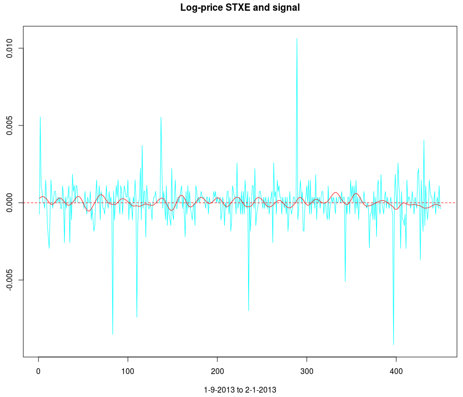
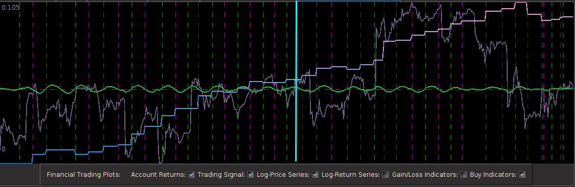
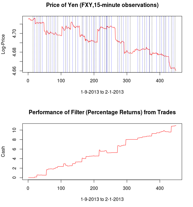
 and the coefficients decay beautifully with perfect smoothness achieved. Notice the two transfer functions perfectly picking out the spectral peak that is intrinsic to the close-to-open cycle that I mentioned was between .23 and .32. To verify these filter coefficients achieve the extraction of the close-to-open cycle, I compute the trading signal from the imdfa object and then plot it against the log-returns of STXE. I then compute the trades in-sample using the signal and the log-price of STXE. The R code is below and the plots are shown in Figures 5 and 6.
 to a low-pass filter with cutoff set at
  , I then computed the filter with the new lowpass design. The transfer functions for the filter coefficients are shown below in Figure 11, with the red colored plot the transfer function for the STXE. Notice that the transfer function for the explanatory series still privileges spectral peak between .23 and .32, with only a slight lift at frequency zero (compare this with the bandpass design in Figure 4, not much has changed). The problem is that the peak exceeds 1.0 in the passband, and this will amplify the cyclical component extracted from the log-return. It might be okay, trading wise, but not what I’m looking to do. For the STXE filter, we get slightly more of a lift at frequency zero, however this has been compensated with a decreased cycle extraction between frequencies .23 and .32. Also, a slight amount of noise has entered in the stopband, another factor we must mollify.
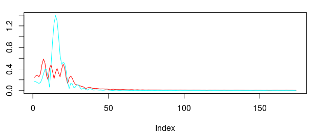
 is one. After doing this, I get the following transfer functions and the respective filter coefficients.
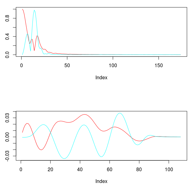

 . Once the bandpass target
  ,
,  , and
, and  .
.
 .
.
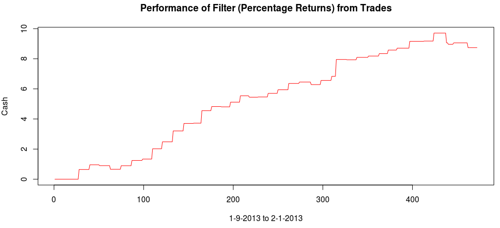
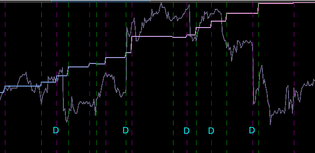
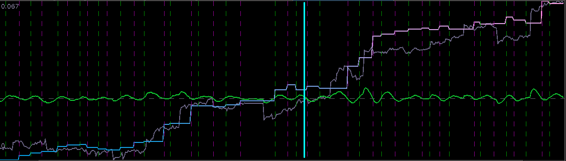
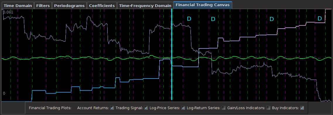
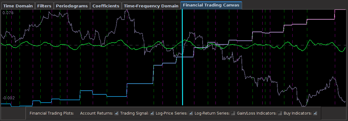
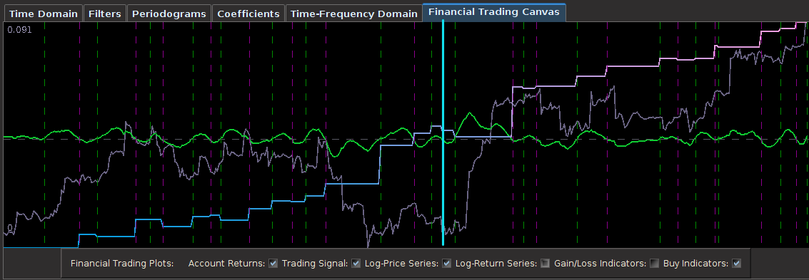
 from the band-pass design and setting the lower cutoff to 0. I also increased the smoothing parameter to $\alpha = 32$. In this newly designed filter, we see a vast improvement in the trading structure. As before, the filter was able to deduce the direction of every single close-to-open jump during the 200 out-of-sample observations, but notice that it was also able to become much more flexible in the trading during any upswing/downswing and volatile period. This is seen in more detail in Figure 7, where I added the letter ‘D’ to each of the 5 major buy/sell signals occurring before close.
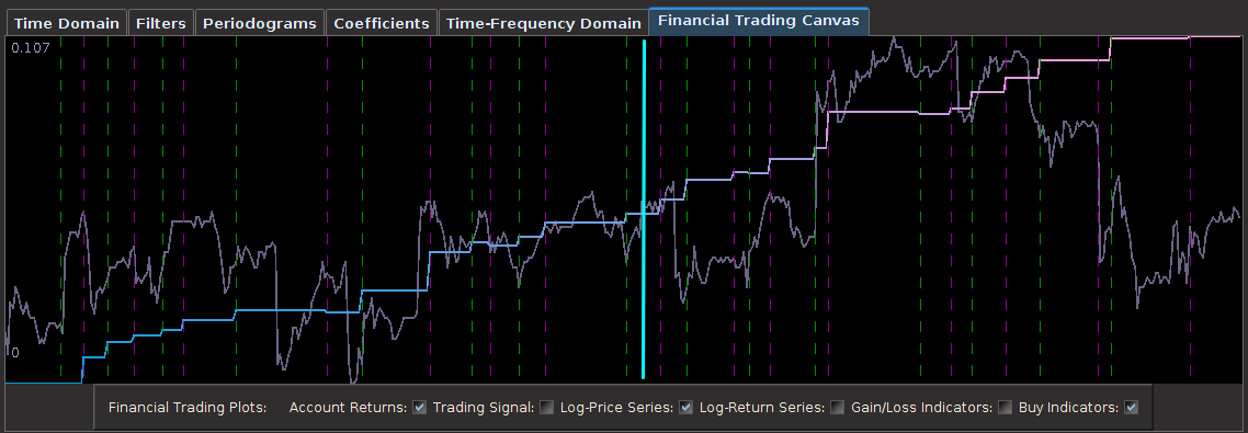
 , down from
  as I had on the band-pass filter. This allows for slightly higher frequencies than
 , I then set the regularization parameters to be
  ,
, 
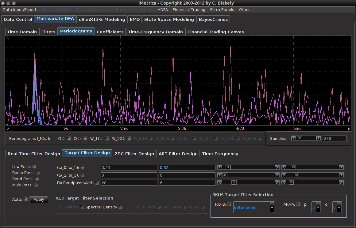
 . Notice that both cutoffs are set directly after a spectral peak, something that I highly recommend. In high-frequency trading on the FOREX using MDFA, as we’ll see, the trick is to seek out the spectral peak which accounts for the close-to-open variation in the price of the foreign currency. We want to take advantage of this spectral peak as this is where the big gains in foreign currency trading using MDFA will occur.
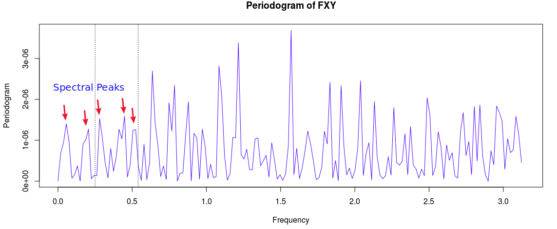
 and expweight to 0 along with setting all the regularization parameters to 0 as well. This will give me a barometer for where and how much to adjust the filter parameters. In selecting the filter length
  , my empirical studies over numerous experiments in building trading signals using iMetrica have demonstrated that a ‘good’ choice is anywhere between 1/4 and 1/5 of the total in-sample length of the time series data. Of course, the length depends on the frequency of the data observations (i.e. 15 minute, hourly, daily, etc.), but in general you will most likely never need more than
  which I’ll stick to for the remainder of this tutorial. In any case, the length of the filter is not the most crucial parameter to consider in building good trading signals. For a good robust selection of the filter parameters couple with appropriate explanatory series, the results of the trading signal with
  compared with, say,
  should hardly differ. If they do, then the parameterization is not robust enough.
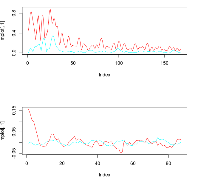
 and expweight customization parameters however need to be adjusted to account for the new noise suppression requirements in the stopband and the phase properties in the smaller passband. Thus I increase the smoothing parameter and decreased the timeliness parameter (which only affects the passband) to account for this change. The new frequency response functions and filter coefficients for this smaller lowpass design are shown below in Figure 11. Notice that the second spectral peak is accounted for and only slightly mollified under the new changes. The coefficients still have the noticeable smoothness and decay at the largest lags.
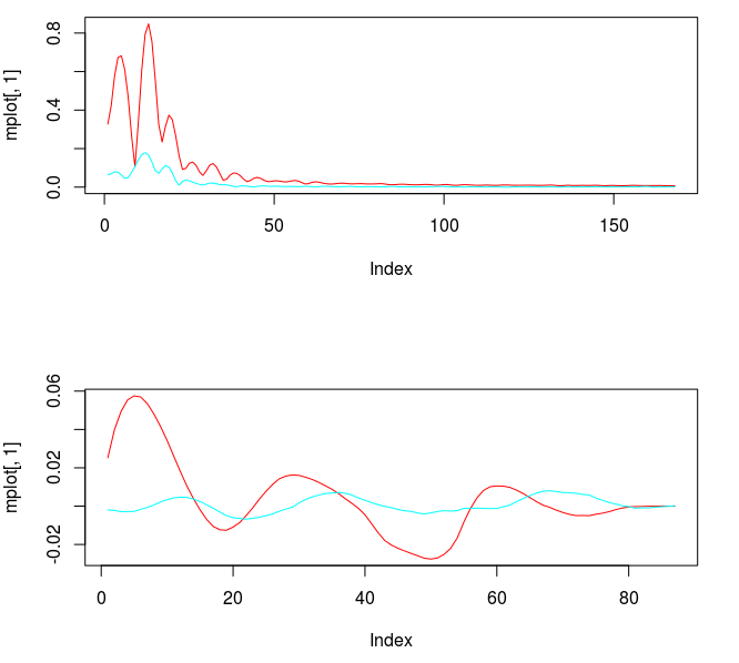

 = 13.2,

 , but this is typically normal and a non-issue. I had to balance for both timeliness and smoothness in this filter using both the customization parameters
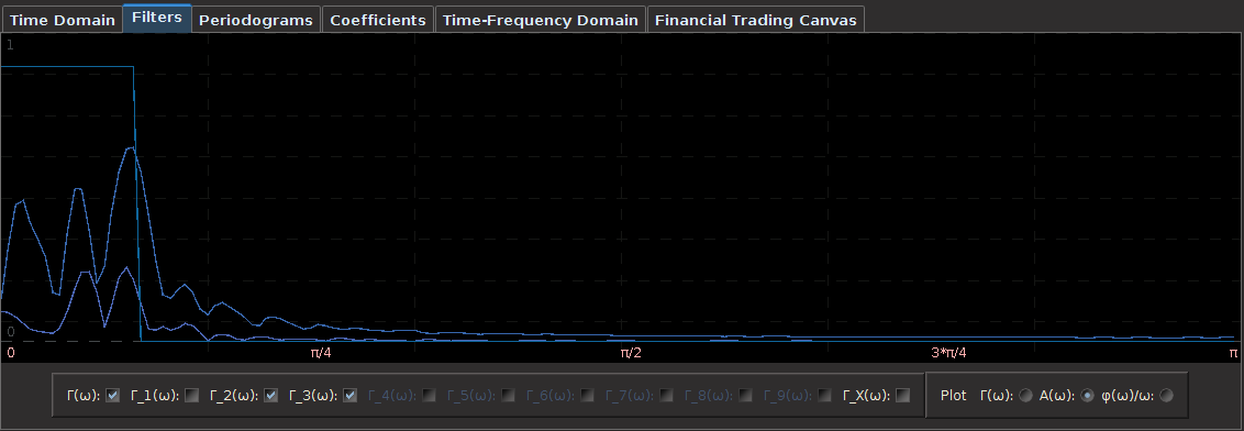


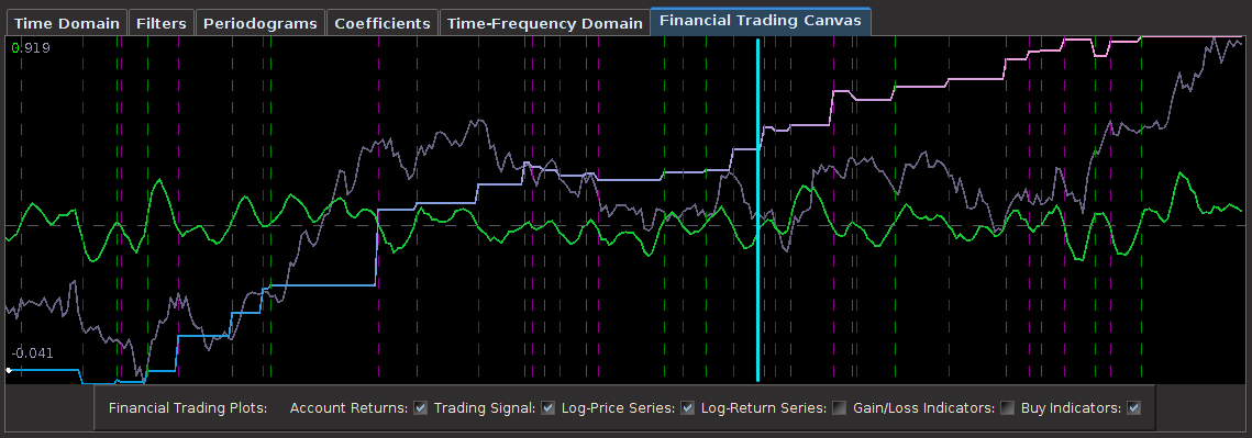


 (see my previous two articles on The Frequency Effect). Designating a lowpass or bandpass filter in the frequency domain will give an indication of what kind of patterns the extracted trading signal will trade on. Traditionally one can set a lowpass with the goal of extracting trends (with the proper amount of timeliness prioritized in the parameterization), or one can opt for a bandpass to extract smaller cyclical events for more systematic trading during volatile periods. But now suppose we could have the best of both worlds at the same time. Namely, be profitable in both steady climbs and long tumbles, while at the same time systematically hacking our way through rough sideways volatile territory, making trades at specific frequencies embedded in the share price actions not found in long trends. The answer is through the construction of multi-band pass filters. Their construction is relatively simple, but as I will demonstrate in this article with many examples, they are a bit more difficult to pinpoint optimally (but it can be done, and the results are beautiful… both aesthetically and financially).
![A := 1_{[\omega_0, \omega_1]}](https://s0.wp.com/latex.php?latex=A+%3A%3D+1_%7B%5B%5Comega_0%2C+%5Comega_1%5D%7D&bg=ffffff&fg=323232&s=0&c=20201002) ,
, ![B := 1_{[\omega_2, \omega_3]}](https://s0.wp.com/latex.php?latex=B+%3A%3D+1_%7B%5B%5Comega_2%2C+%5Comega_3%5D%7D&bg=ffffff&fg=323232&s=0&c=20201002) with
with  and
and  , zero everywhere else, it is easy to see that the motivation here is to seek a detection of both lower frequencies and low-mid frequencies in the data concurrently. With now up to four cutoff frequencies to choose from, this adds yet another few wrinkles in the degrees of freedom in parameterizing the MDFA setup. If choosing and optimizing one cutoff frequency for a simple low-pass filter in addition to customization and regularization parameters wasn’t enough, now imagine extracting signals with the addition of up to three more cutoff frequencies. Despite these additional degrees of freedom in frequency interval selection, I will later give a couple of useful hacks that I’ve found helpful to get one started down the right path toward successful extraction.
 for
for  that acts on the periodogram (or discrete Fourier transforms in multivariate mode) is now defined piecewise according to the different intervals
 ![[0,\omega_0]](https://s0.wp.com/latex.php?latex=%5B0%2C%5Comega_0%5D&bg=ffffff&fg=323232&s=0&c=20201002) ,
, ![[\omega_1, \omega_2]](https://s0.wp.com/latex.php?latex=%5B%5Comega_1%2C+%5Comega_2%5D&bg=ffffff&fg=323232&s=0&c=20201002) , and
, and ![[\omega_3, \pi]](https://s0.wp.com/latex.php?latex=%5B%5Comega_3%2C+%5Cpi%5D&bg=ffffff&fg=323232&s=0&c=20201002) . For example,
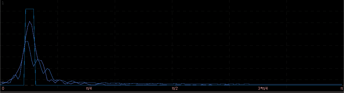
. For example,  gives a piecewise quadratic weighting function (an example shown in Figure 1) and for
  , the weighting function is piecewise linear. In practice, the piecewise power function smooths and rids of unwanted frequencies in the stop band much better than using a piecewise constant function. With these preliminaries defined, we now move on to the first steps in building and applying multiband pass filters.
 if
if ![\omega \in [0,.17]](https://s0.wp.com/latex.php?latex=%5Comega+%5Cin+%5B0%2C.17%5D&bg=ffffff&fg=323232&s=0&c=20201002) , and 0 otherwise. This formulation, as it includes the zero frequency, should provide a local bias as well as extract very slow moving trends. The trick with these filters for building consistent trading performance is ensure a proper grip on the timeliness characteristics of the filter in a very low and narrow filter passage. Regularization and smoothness using the weighting function shouldn’t be too much of a problem or priority as typically just only a small fraction of the available degrees of freedom on the frequency domain are being utilized, so not much concern for overfitting as long as you’re not using too long of a filter. In my example, I maxed out the timeliness
, and 0 otherwise. This formulation, as it includes the zero frequency, should provide a local bias as well as extract very slow moving trends. The trick with these filters for building consistent trading performance is ensure a proper grip on the timeliness characteristics of the filter in a very low and narrow filter passage. Regularization and smoothness using the weighting function shouldn’t be too much of a problem or priority as typically just only a small fraction of the available degrees of freedom on the frequency domain are being utilized, so not much concern for overfitting as long as you’re not using too long of a filter. In my example, I maxed out the timeliness  regularization parameter to .3. Fortunately, no optimization of any parameter was needed in this example, as the performance was spiffy enough nearly right after gauging the timeliness parameter
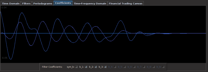
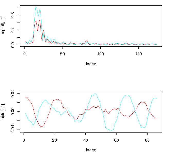
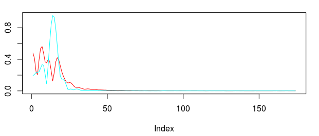
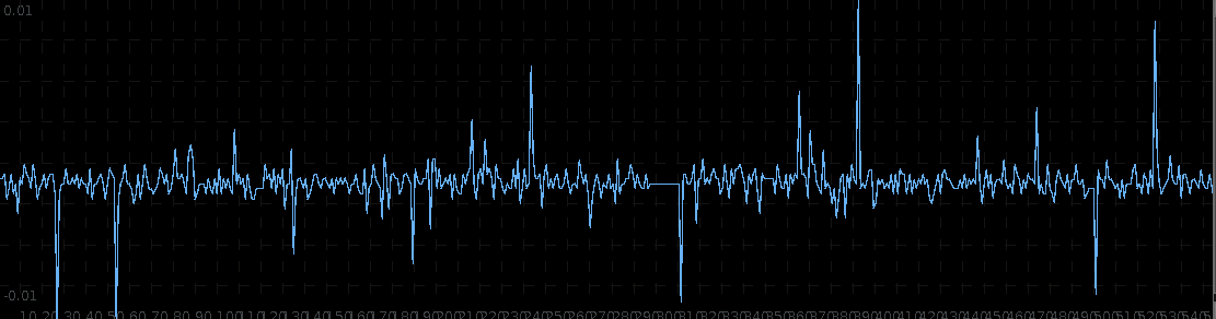
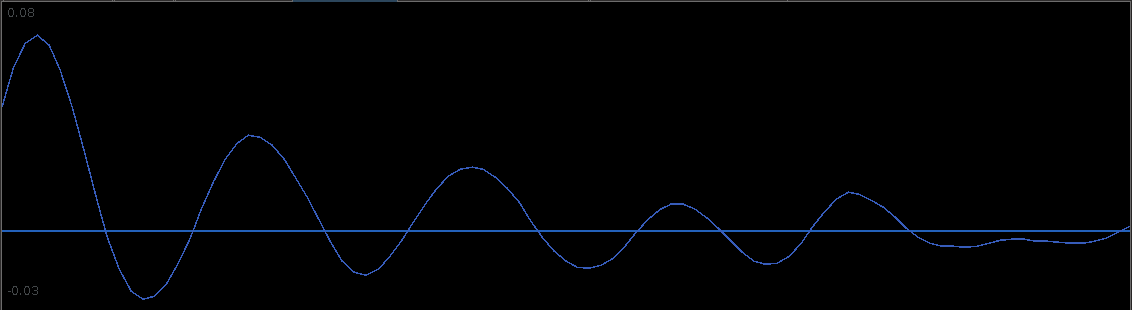
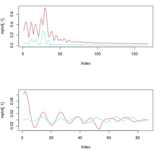
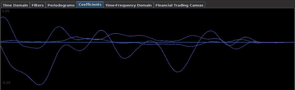
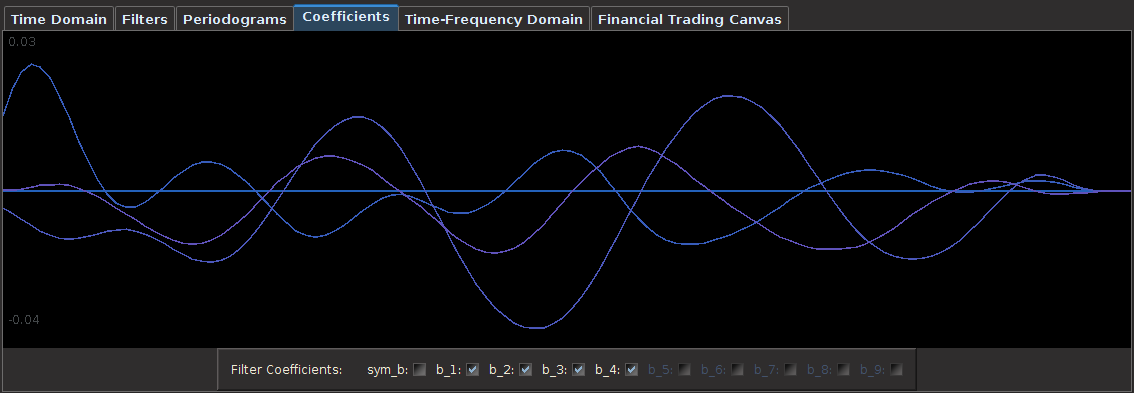
 for both the sets of explanatory log-return data and Figure 4 depicts the coefficients for the filter. Notice that in the coefficients plot, much more weight is being assigned to past values of the log-return data with extreme (min and max values) at around lags 15 and 30 for the GOOG coefficients (blue-ish line). The coefficients are also quite smooth due to the slight amount of smooth regularization imposed.

 is highly dependent on the data and should be located through a priori investigations (as I did above, without the additional bandpass).
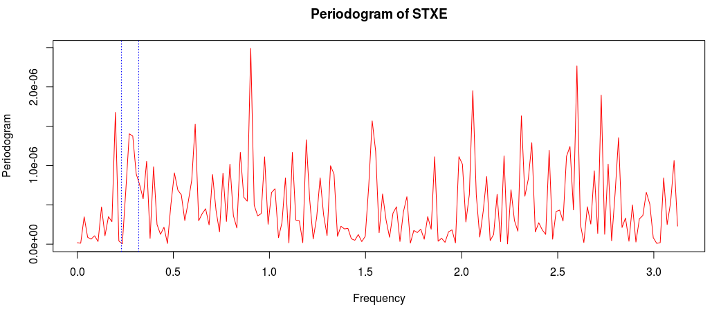
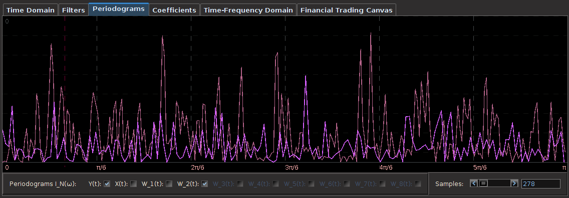
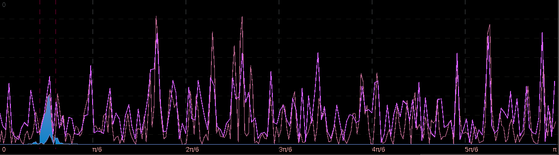
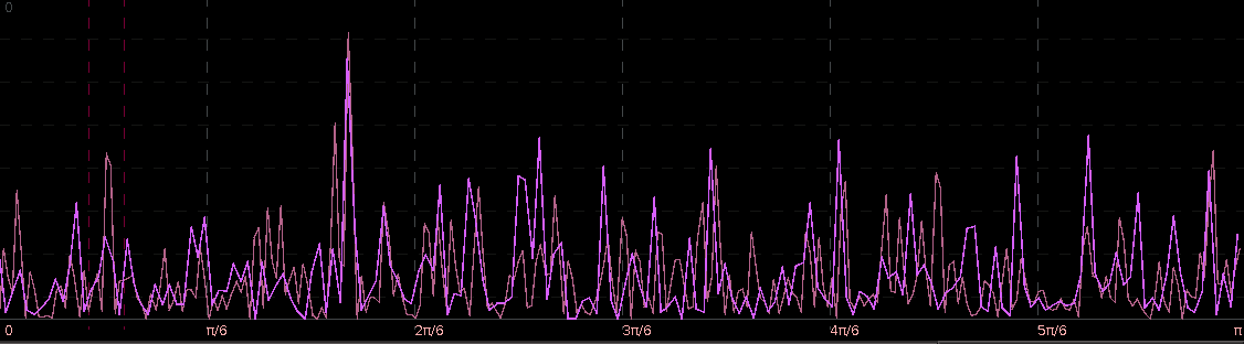
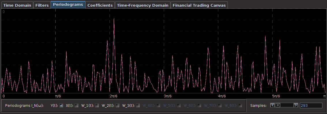
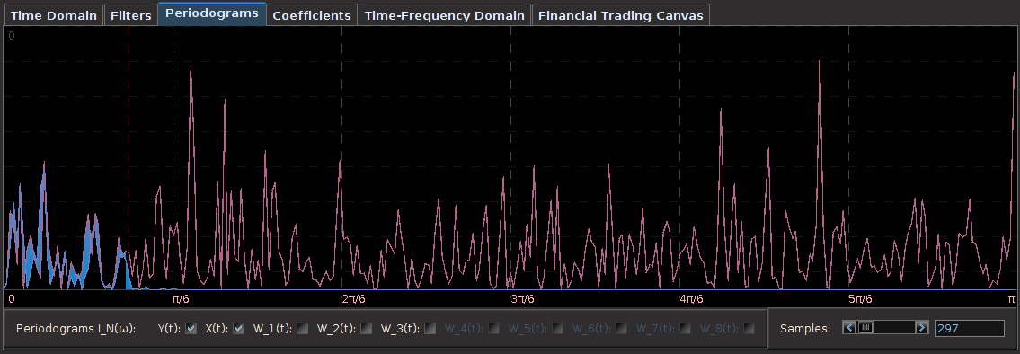
 . The largest of these peaks will be defined from here on out as the principal spectral peak (PSP). Figure 6 shows an example of an averaged periodogram of the log-return for GOOG and AAPL with the PSP indicated. You might note that there exists a much larger spectral peak located at
  , but no need to worry about that one (unless you really enjoy transaction costs). I locate this PSP as a starting point for where I want my signal to trade.
![[.49,.65]](https://s0.wp.com/latex.php?latex=%5B.49%2C.65%5D&bg=ffffff&fg=323232&s=0&c=20201002) with the PSP directly under it. I then optimized the regularization controls in-sample (a feature I haven’t discussed yet) and slightly tweaked the timeliness parameter (ended up setting it to 3) and my result (drumroll…) is shown in Figure 6.
with the PSP directly under it. I then optimized the regularization controls in-sample (a feature I haven’t discussed yet) and slightly tweaked the timeliness parameter (ended up setting it to 3) and my result (drumroll…) is shown in Figure 6.
![[.51, .68]](https://s0.wp.com/latex.php?latex=%5B.51%2C+.68%5D&bg=ffffff&fg=323232&s=0&c=20201002) , with the PSP still underneath the bandpass, but now catching on to a few more higher frequencies then before. I also slightly increased the length of the filter to see if that had any affect. After optimizing on the timeliness parameter
, with the PSP still underneath the bandpass, but now catching on to a few more higher frequencies then before. I also slightly increased the length of the filter to see if that had any affect. After optimizing on the timeliness parameter 


![(\omega_0, \omega_1) \subset [0,\pi]](https://s0.wp.com/latex.php?latex=%28%5Comega_0%2C+%5Comega_1%29+%5Csubset+%5B0%2C%5Cpi%5D&bg=ffffff&fg=323232&s=0&c=20201002) where
where  . We can introduce a constraint on the filter coefficients so as to impose a vanishing time-shift at frequency zero. As Wildi says on page 24 of the Elements paper: “A vanishing time-shift is highly desirable because turning-points in the filtered series are concomitant with turning-points in the original data.” In fact, we can take this a step further and even impose an arbitrary time-shift with the value
  at frequency zero, where
  at zero is
  , which implies
  .
.